Olkkonen J. (ed.) Discrete Wavelet Transforms - Theory and Applications
Подождите немного. Документ загружается.


However, this is not possible, because there is a direct trade off between time and
frequency resolution of basis functions as gov erned by the Heisenburg uncertainty principal
Burrus et al. (1998) Mallat (1998). The Heisenburg uncertainty principal states that resolution
of the time-frequency functions are lower bounded by
Δω
·Δt ≥ 1/2. (10)
Therefore, to capture nonstationary events with good space-frequency localization, we need
basis functions that aim to o perate near the theoretical lower bound. Many basis functions
offer solutions, but are not optimal for all applications. For example, the Short-Time Fourier
Transform (STFT) bases are not optimal because (1) they offer a fixed resolution for the
entire decomposition process (thus missing features that are comprised with different scales
and frequencies) , (2) do not offer an easy m ethod to access and manage the coefficients
and (3) creates a drastic increase in memory consumption and computational resources.
The following section will describe how the wavelet transform poses solutions to all these
problems.
4.2 Wavelet transforms
The wavelet transform offers solutions to all the problems associated with other basis
functions (such as the ST FT) Mallat (1989) Wang & Karayiannis (1998) Vetterli & Herley
(1992) Mallat (1998). It offers a multiresolutional representation (decomp oses the image using
various scale-frequency resolutions), which is achieved by dyadically changing the size of the
window. Space-frequency events are localized with good results since the changing window
function is tuned to events which have high frequency components in a small analysis
window (scale) or low frequency events with a large scale Burrus et al. (1998) . Therefore,
texture events could be efficiently represented using a set of multiresolutional basis functions.
Additionally, the discrete wavelet transform utilizes critical subsampling along rows and
columns and uses these subsampled subbands as the input to the next decomposition level.
For a 2-D image, this reduces the number of input samples by a factor of four for each level of
decomposition. This representation may be stored back on to the original image for minimum
memory usage and it also permits for an organized, computationally efficient manner to
access these subbands and extract meaningful features.
The wavelet transform utilizes both wavelet basis ψ
j,k
(t) and scaling basis φ
k
(t) functions.
The wavelet functions are used to localize the hi gh frequency content, whereas the scaling
function examines the low frequencies. The scale of the analysis window changes with each
decomposition level, thus achieving a multiresolutional representation. Starting with the
initial scale j
= 0, the wavelet transform of any function f (t) which belongs to L
2
(R) is found
by
f
(t)=
k=∞
∑
k=−∞
c(k) · φ
k
(t)+
j=∞
∑
j=0
k
=∞
∑
k=−∞
d(j, k) ·ψ
j,k
(t) , (11)
where c
(k) are the scaling or aver aging co efficients (low frequency material) defined by
c
(k)=c
0
(k)=�f (t), φ
k
(t)� =
f (t)φ
k
(t) dt, (12)
and d
j
(k) are the detail wavelet coefficients (high frequency content) defined by
d
j
(k)=d(j, k)=�f (t), ψ
j,k
(t)� =
f (t)ψ
j,k
(t) dt. (13)
In o rder to achieve a wavelet transform, the functions ψ
j,k
(t) and φ
k
(t) have to meet specific
criteria. These criteria, the properties of the scaling/wavelet functions and the corresponding
sig nal spaces are described next.
4.2.1 Scaling funct ion subspaces
Consider a set of basis functions {φ
k
(t)} which may be created by translating the prototype
scaling function φ
(t) Burrus et al. (1998)
φ
k
(t)=φ(t − k), k ∈ Z, (14)
where φ
k
(t) spans the space V
o
V
o
= Span
k
{φ
k
(t)}. (15)
If a set of basis functions span a signal space
V
o
, then any function f (t) which also belongs to
that space can be completely represented using those basis functions as in: f
(t)=
∑
k
a
k
·φ
k
(t)
(for any f (t) ∈V
o
).
For added flexibility, the time and frequency resolution of these scaling functions may be
adjusted by including an additional s cale parameter j in the characteristic basis functi on
expression
φ
j,k
(t)=2
j/2
·φ(2
j
t − k), j, k ∈ Z, (16)
where the scalar multiple 2
j/2
is incl uded to ensure orthonormality Mallat (1989). Therefore,
an entire series of basis functions can be created by simply dilating (changing the j value) or
translating (changing the k value) the prototyp e scaling function φ
(t) . These basis functions
span the subspace
V
j
V
j
= Span
k
{φ
k
(2
j
t )},
= Span
k
{φ
j,k
(t)}, (17)
and any signal f
(t) can be expressed using this expansion set, as long as it is also a set of V
j
f (t)=
∑
k
a
k
·φ(2
j
t − k), f (t) ∈V
j
. (18)
The i ntroduction of a scale parameter change s the time duration of the scaling f unctions.
This allows different resolutions to isolate different anomalies in the signals or images. For
instance, if j
> 0, φ
j,k
(t) is narrower and would provide a good representation of finer
detail. For j
< 0, the basis functions φ
j,k
(t) are wider and would be ideal to represent coarse
information Burrus et al. (1998).
4.2.2 Wavelet basis functions
Although the scali ng functio ns give way to a multi resolution representation, it i s also
necess ary to investigate the spaces which span the differences of the spaces spanned by the
scali ng functions. These regions correspond to the high frequency details of the data.
189
Shift-Invariant DWT for Medical Image Classification
......
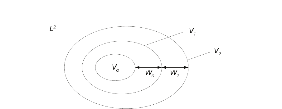
Fig. 4. Nested wavelet and scaling signal spaces.
The types of basis functions that can localize the details are known as wavelets ψ
(t) and their
corresponding signal spaces are denoted as
W. Similar to s caling functions, a series of wavelet
basis functions can be generated by dilating and translating the mother wavelet ψ
(t)
ψ
j,k
(t)=2
j/2
ψ(2
j
t − k), j, k ∈ Z. (19)
To find the mother wavelet ψ(t), it is necessary to find the relationship between the mother
wavelet ψ
(t) and the g enerating scaling function φ(t).
Starting with an initial resolution of j
= 0, the nested subspaces may be written as
V
o
⊂V
1
⊂V
2
⊂···⊂L
2
. (20)
The corresponding spaces spanned by the wavelet basis functions are shown in Figure 4,
which illustrates how each
W subspace spans the difference of two subspaces. As shown in
Figure 4, the signal spaces
V
1
and V
2
may be expressed as
V
1
= V
o
⊕W
o
, (21)
and
V
2
= V
o
⊕W
o
⊕W
1
, (22)
where
⊕ is a direct sum. If V
j
is the space spanned by the scaling functions φ
j,k
(t) and
V
j+1
is the space spanned by the functions φ
j+1,k
(t) , then W
j
is the disjoint difference or the
orthogonal compliments of
V
j
and V
j+1
spanned by the wavelet basis functions ψ
j,k
(t) . This
may be shown by
V
j+1
= V
j
⊕W
j
, ∀j ∈ Z. (23)
Using Equation 21, Equation 22 and Figure 4, a general expression for the L
2
subspace may be
developed:
L
2
= V
o
⊕W
o
⊕W
1
⊕W
2
⊕···, (24)
and since thes e subspaces are orthogonal to one another
V
o
⊥W
o
⊥W
1
⊥W
2
⊥W
3
···, (25)
190
Discrete Wavelet Transforms - Theory and Applications

......
Fig. 4. Nested wavelet and scaling signal spaces.
The types of basis functions that can localize the details are known as wavelets ψ
(t) and their
corresponding signal spaces are denoted as
W. Similar to s caling functions, a series of wavelet
basis functions can be generated by dilating and translating the mother wavelet ψ
(t)
ψ
j,k
(t)=2
j/2
ψ(2
j
t − k), j, k ∈ Z. (19)
To find the mother wavelet ψ(t), it is necessary to find the relationship between the mother
wavelet ψ
(t) and the g enerating scaling function φ(t).
Starting with an initial resolution of j
= 0, the nested subspaces may be written as
V
o
⊂V
1
⊂V
2
⊂···⊂L
2
. (20)
The corresponding spaces spanned by the wavelet basis functions are shown in Figure 4,
which illustrates how each
W subspace spans the difference of two subspaces. As shown in
Figure 4, the signal spaces
V
1
and V
2
may be expressed as
V
1
= V
o
⊕W
o
, (21)
and
V
2
= V
o
⊕W
o
⊕W
1
, (22)
where
⊕ is a direct sum. If V
j
is the space spanned by the scaling functions φ
j,k
(t) and
V
j+1
is the space spanned by the functions φ
j+1,k
(t) , then W
j
is the disjoint difference or the
orthogonal compliments of
V
j
and V
j+1
spanned by the wavelet basis functions ψ
j,k
(t) . This
may be shown by
V
j+1
= V
j
⊕W
j
, ∀j ∈ Z. (23)
Using Equation 21, Equation 22 and Figure 4, a general expression for the L
2
subspace may be
developed:
L
2
= V
o
⊕W
o
⊕W
1
⊕W
2
⊕···, (24)
and since thes e subspaces are orthogonal to one another
V
o
⊥W
o
⊥W
1
⊥W
2
⊥W
3
···, (25)
the corresponding basis functions which span t hese spaces are also orthogonal
�φ
j,k
(t) , ψ
j,k
(t)� =
φ
j,k
(t) · ψ
j,k
(t)dt = 0. (26)
Furthermore, wavelet spaces at a scale j are a subset of the scale spaces at the next scale j
+ 1
W
j
⊂V
j+1
. (27)
Consequently, wavelets reside in the space spanned by the next narrower scal ing function and
can be expressed as a weighted sum of shifted scaling functions, φ
(2t)
ψ(t)=
∑
n
h
1
(n) ·
√
2 ·φ(2t − n ), n ∈ Z, (28)
where h
1
(n) are the wavelets’ coefficients. Equation 28 shows that the generating wavelet
ψ
(t) can be produced from the prototype scaling function φ(t) by choosing the appropriate
h
1
(n). In order to ensure orthogonality, the scaling and wavelet coefficients must be related
by Burrus et al. (1998)
h
1
(n)=(−1)
n
h
o
(1 − n). (29)
Therefore, for analysis with orthogonal wavelets, the highpass filter h
1
(n), which is half-band,
is calculated as the quadrature mirror filter of the lowpass h
o
(n). These filters may be
used to efficiently implement the wavelet transform for discrete signals (the Discrete Wavelet
Transform) and is discussed next.
4.3 Discrete wavelet transform
In order to perform the wavelet transform for discrete images, implementation of the DWT
using filterbanks is popular choice since the complex ities of the wavelet transform are
explained in terms of filtering operations (which is intuitive). The material is first presented
for one dimensional signals and then is expanded to 2D for images.
After performi ng a series of simplifications and change of vari ables Burrus et al. (1998) Mallat
(1998) Vetterl i & Herley (1992), Equ ation 28 may be re w ritten as
c
j
(k)=
∑
m
h
o
(m −2k)c
j+1
(m), (30)
and
d
j
(k)=
∑
m
h
1
(m −2k)c
j+1
(m). (31)
This illustrates that c
j
(k) and d
j
(k) can be found by filtering c
j+1
(k) with h
o
and h
1
,
respectively, followed by a decimation by a factor of 2. The two filters, h
o
(n) and h
1
(n)
are half-band lowpass and highpass filters, respectively. C onsequently, the lowpass filter
h
o
(n) produces lowpassed or averaged coefficients c
j
(k) and the highpass filter h
1
(n) creates
highpassed or detail coefficients d
j
(k).
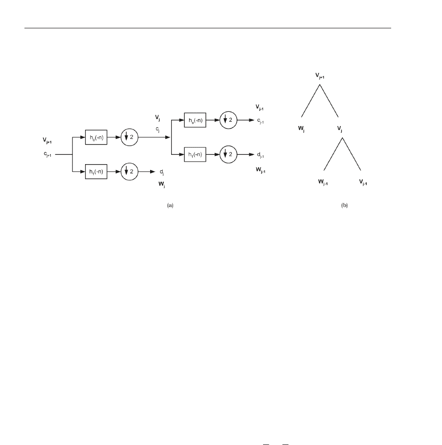
To compute the DWT coefficients for two levels, examine the two stage analysis filterbank in
Figure 5(a) alongside the signal spaces in Figure 5(b). Note that the initial scale here is j
+ 1,
and there fore c
j+1
would represent the original input signal. After one level of decomposition,
the lowpass coefficients c
j
and the highpas s details d
j
are produced. For a multiresolutional
representation, c
j
are further decompo sed with h
o
and h
1
, to produce the coefficients c
j−1
(k)
191
Shift-Invariant DWT for Medical Image Classification
and d
j−1
(k) (they describe the next scale of low and high frequency structures). The 2D
extension for images is detailed next.
Fig. 5. (a) Computing the 1-D wavelet and scaling coefficients using filtering and decimation
with a 2-stage analysis filterbank, (b) corresponding decomposition tree showing the division
of signal spaces.
4.3.1 2-D extension for images
Instead of having a wavelet or filter which is a function of the two spatial dimensions of an
image, the filter can be separable, which allows a particular 1D filter to be applied to the rows
and columns of an im age separately to gain the desired overall 2D response Lawson & Zhu
(2004). A separable filte r for two dimensions may be denoted by:
H
(z
1
, z
2
)=H(z
1
) · H(z
2
), (32)
where z
1
and z
2
relate to the spatial dimensions of an image. Therefore, the filters defined
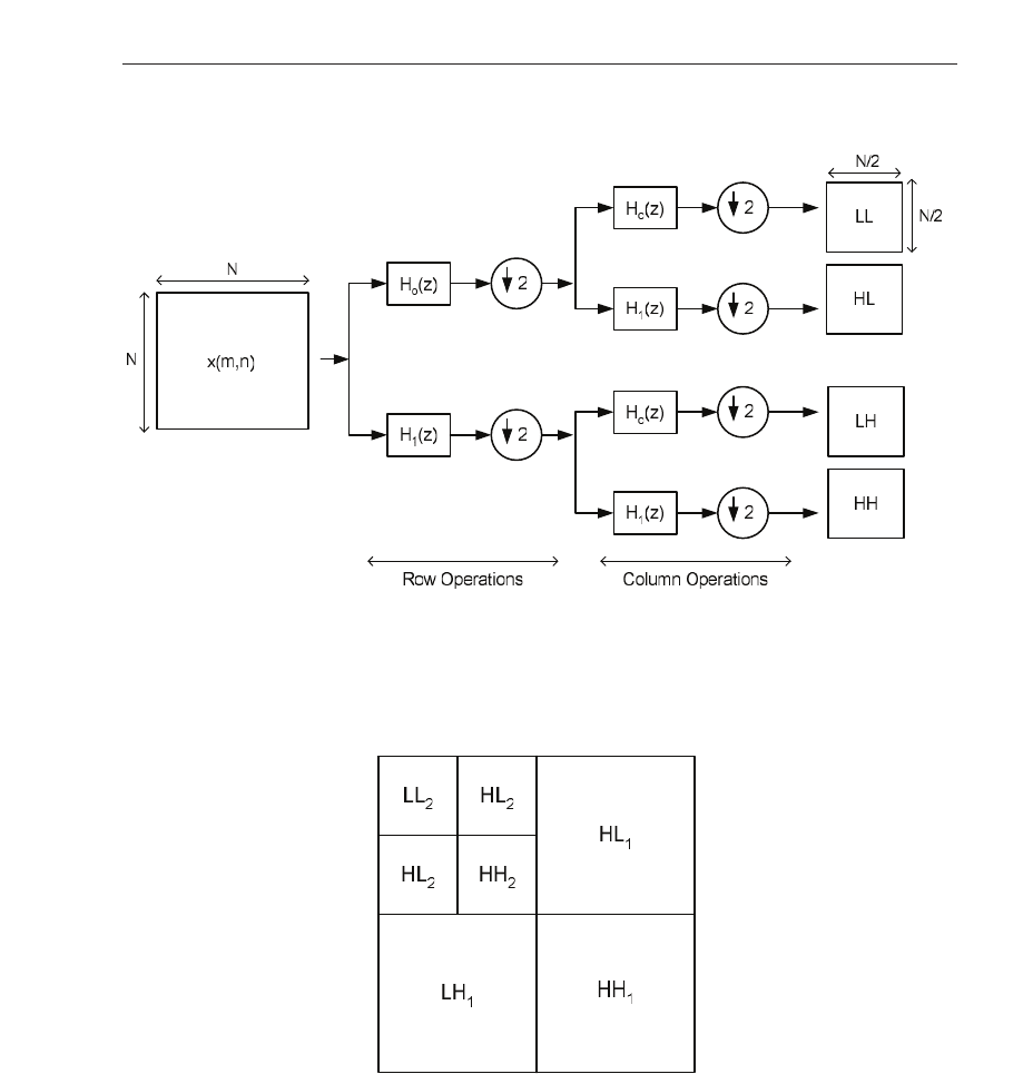
for the 1D DWT may be applied separably to gain a 2D DWT representation for images. The
2-D DWT filterbank scheme for an N
× N image x(m, n) is shown in Figure 6. Initially, the
filters H
o
(z) and H
1
(z) are applied to the rows of image x(m, n), creating two images which
respectively contain the low and high frequency conte nt of the image in question. After this,
both fre quency bands are subsampled by a factor of 2, and are sent to the next set of filters for
filtering along the columns. After these bands have been filtered, decimation by a factor of 2
is again performed, but this time along columns. At the output of one level of decomposition,
as shown in Figure 6, there are four subband images o f size
N
2
×
N
2
labeled LL, LH, HL and
HH. Using the separability concept, at scale j, these subbands may be computed by
LL
j
(x, y)=
∑
m
∑
n
h
o
(m −2x)h
o
(n −2y) · LL
j+1
(m, n), (33)
HL
j
(x, y)=
∑
m
∑
n
h
o
(m −2x)h
1
(n −2y) · LL
j+1
(m, n), (34)
LH
j
(x, y)=
∑
m
∑
n
h
1
(m −2x)h
o
(n −2y) · LL
j+1
(m, n), (35)
HH
j
(x, y)=
∑
m
∑
n
h
1
(m −2x)h
1
(n −2y) · LL
j+1
(m, n). (36)
192
Discrete Wavelet Transforms - Theory and Applications
and d
j−1
(k) (they describe the next scale of low and high frequency structures). The 2D
extension for images is detailed next.
Fig. 5. (a) Computing the 1-D wavelet and scaling coefficients using filtering and decimation
with a 2-stage analysis filterbank, (b) corresponding decomposition tree showing the division
of signal spaces.
4.3.1 2-D extension for images
Instead of having a wavelet or filter which is a function of the two spatial dimensions of an
image, the filter can be separable, which allows a particular 1D filter to be applied to the rows
and columns of an im age separately to gain the desired overall 2D response Lawson & Zhu
(2004). A separable filte r for two dimensions may be denoted by:
H
(z
1
, z
2
)=H(z
1
) · H(z
2
), (32)
where z
1
and z
2
relate to the spatial dimensions of an image. Therefore, the filters defined
for the 1D DWT may be applied separably to gain a 2D DWT representation for images. The
2-D DWT filterbank scheme for an N
× N image x(m, n) is shown in Figure 6. Initially, the
filters H
o
(z) and H
1
(z) are applied to the rows of image x(m, n), creating two images which
respectively contain the low and high frequency conte nt of the image in question. After this,
both fre quency bands are subsampled by a factor of 2, and are sent to the next set of filters for
filtering along the columns. After these bands have been filtered, decimation by a factor of 2
is again performed, but this time along columns. At the output of one level of decomposition,
as shown in Figure 6, there are four subband images o f size
N
2
×
N
2
labeled LL, LH, HL and
HH. Using the separability concept, at scale j, these subbands may be computed by
LL
j
(x, y)=
∑
m
∑
n
h
o
(m −2x)h
o
(n −2y) · LL
j+1
(m, n), (33)
HL
j
(x, y)=
∑
m
∑
n
h
o
(m −2x)h
1
(n −2y) · LL
j+1
(m, n), (34)
LH
j
(x, y)=
∑
m
∑
n
h
1
(m −2x)h
o
(n −2y) · LL
j+1
(m, n), (35)
HH
j
(x, y)=
∑
m
∑
n
h
1
(m −2x)h
1
(n −2y) · LL
j+1
(m, n). (36)
The first letter of the subimages indicates the operation that was performed on the columns
(i.e. L is for lowpass filtering with H
o
(z) and H is for highpass filtering with H
1
(z))
whereas the last letter indicates which operation was performed on the rows. If more levels
Fig. 6. Filterbank implementation of 2-D discrete wavelet transform (DWT).
of decomposition are required, the LL band may be recursively reapplied to the analysis
filterbank of Figure 6. For two levels of decomposition, the placement of the coefficients back
onto the image is shown in Figure 7.
To examine the localization properties of the 2D DWT, consider Figure 8. The edges and
Fig. 7. Graphical depiction of wavelet coefficient placement for two levels of decomposition.
corners of the square (the original image) are composed of localized high frequency content,
which is captured in the high frequency subbands in the wavelet domain, re gardl ess of the
orientation (horizontal, diagonal, vertical). As texture is comprised of such localized high
frequency events, util ization of such a transform will be able to describe the textural events
as required. The diffusion of textural features or events will occur across subbands, which
193
Shift-Invariant DWT for Medical Image Classification
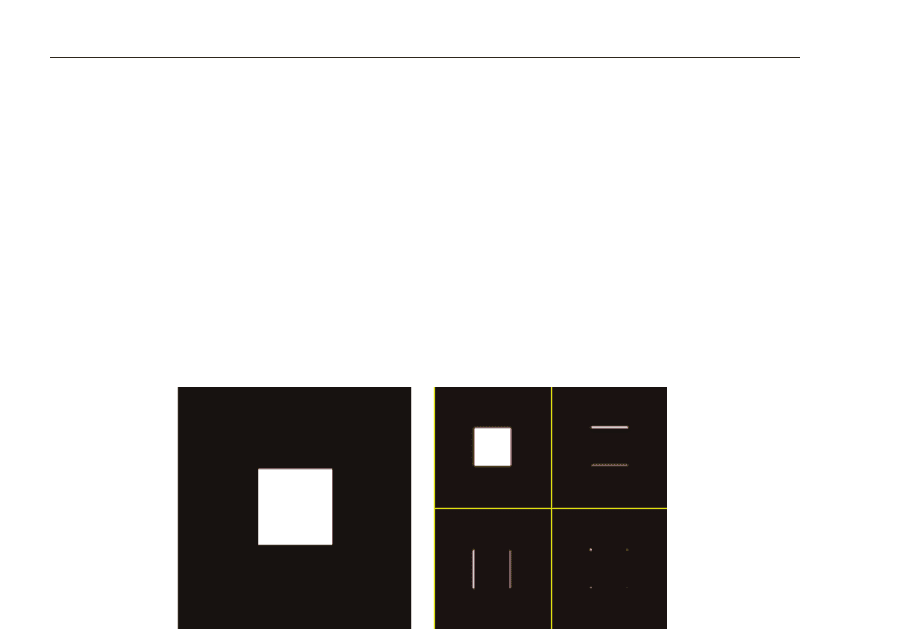
allows features to be captured not only within subbands, but also across subbands.
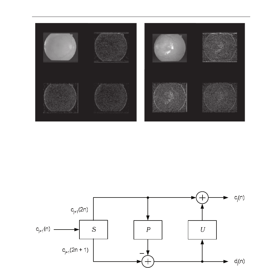
For an example of the localization properties of wavelets in a medical image, as well as
the textural differences between normal and abnormal medical images, see Figure 9. The
normal image’s decomposition ex hibits an overly homogeneous appearance of the wavelet
coefficients in the HH, HL and LH bands (which reflects the uniform nature of the original
image). The de composition of the retinal image with diabeti c retinopathy sho ws that e ach
of the higher frequency subbands localizes the retinopathy, which appears as heterogeneous
textured blobs (high-valued wavelet coefficients) in the center of the subband. This illustrates
how the DWT can localize the textural differences in medical images also how multiscale
texture may be used to discrimi nate between patholog ical cases . Similar results are obtained
with the small bowel and mammographic lesions, however, are not s hown here due to space
constr aints.
Another benefit of wavele t analysis is that the basis functions are scale-invariant.
Fig. 8. Left: original image. Right: one level of DWT of left image.
Scale-invariant basis functions will give rise to a localized description of the texture elements,
regardless of their size or scale, i.e. coarse texture can be made up of large textons, whi le fine
texture is compri sed of smaller elementary u nits. Therefore, the DWT can handle both of these
scenarios.
Although the filterbank method is efficient, it requires a lot of filtering operations which is
computationally expensive. For more efficient implementations of the filterbank-based DWT,
the lifting-based approach is one such approach that is employe d in the current framework
and detailed next.
4.4 Lifting-based DWT
To compute the DWT in an efficient manner, the lifting based app roach is used Fernández
et al. (1996) Sweldens (1995) Sweldens (1996). To increase computation speed, lifting based
approaches make optimal use of similarities which exist between the lowpass (H
1
(z)) and
highpass (H
o
(z)) filters. All 1D implementations will be later extended to 2D implementations
by ’lifting’ both the columns and the rows s eparately.
The lifting based DWT is an efficient scheme since it aims to implement complicated functions
with simple and inverti ble stages Zhang & Zeytinoglu (1999). Compared to the filterbank
method, the lifting based DWT method offers a less computationally expensive solution to
compute the DWT Zhang & Ze ytinoglu (1999) Sweldens (1996).
The lifting based scheme relies on three operations to achieve the discrete wavelet transform:
194
Discrete Wavelet Transforms - Theory and Applications
allows features to be captured not only within subbands, but also across subbands.
For an example of the localization properties of wavelets in a medical image, as well as
the textural differences between normal and abnormal medical images, see Figure 9. The
normal image’s decomposition ex hibits an overly homogeneous appearance of the wavelet
coefficients in the HH, HL and LH bands (which reflects the uniform nature of the original
image). The de composition of the retinal image with diabeti c retinopathy sho ws that e ach
of the higher frequency subbands localizes the retinopathy, which appears as heterogeneous
textured blobs (high-valued wavelet coefficients) in the center of the subband. This illustrates
how the DWT can localize the textural differences in medical images also how multiscale
texture may be used to discrimi nate between patholog ical cases . Similar results are obtained
with the small bowel and mammographic lesions, however, are not s hown here due to space
constr aints.
Another benefit of wavele t analysis is that the basis functions are scale-invariant.
Fig. 8. Left: original image. Right: one level of DWT of left image.
Scale-invariant basis functions will give rise to a localized description of the texture elements,
regardless of their size or scale, i.e. coarse texture can be made up of large textons, whi le fine
texture is compri sed of smaller elementary u nits. Therefore, the DWT can handle both of these
scenarios.
Although the filterbank method is efficient, it requires a lot of filtering operations which is
computationally expensive. For more efficient implementations of the filterbank-based DWT,
the lifting-based approach is one such approach that is employe d in the current framework
and detailed next.
4.4 Lifting-based DWT
To compute the DWT in an efficient manner, the lifting based app roach is used Fernández
et al. (1996) Sweldens (1995) Sweldens (1996). To increase computation speed, lifting based
approaches make optimal use of similarities which exist between the lowpass (H
1
(z)) and
highpass (H
o
(z)) filters. All 1D implementations will be later extended to 2D implementations
by ’lifting’ both the columns and the rows s eparately.
The lifting based DWT is an efficient scheme since it aims to implement complicated functions
with simple and inverti ble stages Zhang & Zeytinoglu (1999). Compared to the filterbank
method, the lifting based DWT method offers a less computationally expensive solution to
compute the DWT Zhang & Ze ytinoglu (1999) Sweldens (1996).
The lifting based scheme relies on three operations to achieve the discrete wavelet transform:
Fig. 9. One level of DWT decomposition of retinal images. Left: normal image
decomposition. Right: decomposition of retinal image with diabetic retinopathy. Contrast
enhancement was performed in the higher frequency bands (HH, LH, HL) for visualization
purposes.
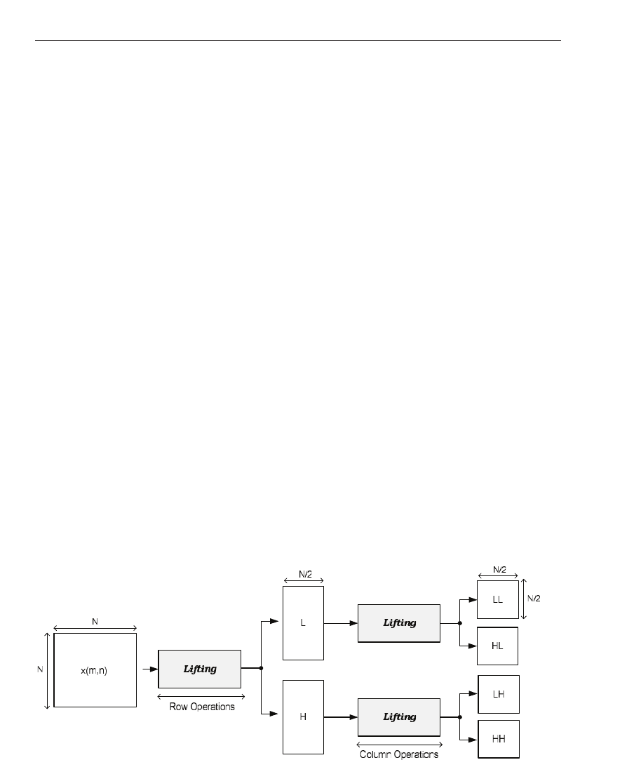
1) split, 2) predict and 3) update. These three operations which comprise the 1-D lifting
scheme, are shown in Figure 10, where
S is the splitting function, P is the predictor f unction
and
U is the update operation. As shown by Figure 10, the scaling and wavelet coefficients
(c
j
(n) and d
j
(n)) are still from the previous level’s coefficients, c
j+1
(n). Lifting may be also
appli ed separably to the rows and columns of an image to arrive at a 2D DWT.
Fig. 10. Generalized 1-D lifting based imple mentation of the DWT.
4.4.1 Splitting
The s plitting operation divides the 1-D input string into even and odd samples, as denoted
by c
j+1
(2n) and c
j+1
(2n + 1), respectively. Using digital signal processing, the even samples
may be obtained by dec imating the original signal by a factor of 2, and the odd samples may
be obtained by subsampling a time shifted (single unit of time) version of the or iginal signal
by 2. This is often referred to as the Lazy Wavelet Transform Fernández et al. (1996).
195
Shift-Invariant DWT for Medical Image Classification
4.4.2 Prediction
In order to compute the wavelet coefficients d
j
(n), a lifting scheme uses a predictor to
interpolate the odd-indexed coefficients from the previous scale (c
j+1
(2n + 1)). The prediction
is subtracted from the original odd-indexed signal to produce the wavelet coefficients d
j
(n).
This may expressed as
d
j
(n)=c
j+1
(2n + 1) −P(c
j+1
(2n + 1)), (37)
where
P(·) is the predictor function. As stated earli er, the wavelet coefficients correspond to
the high frequency components which makes thi s ope ration equivalent to hig hpass filteri ng.
A good predictor function would produce small valued wavelet coefficients (ideally zero),
since the predicted version of the signal would be identical to the original. However, for
nonstationary signals (such as bio medical images) that have properties which change over
time, it is not possible to exactly predict the signal Zhang & Zeytinoglu (1999) and non-zero
wavelet coefficients can be expected. There are many different predictor functions which may
be used Maragos et al. (1984) Haijiang et al. (2004) Denecker et al. (1997), howe ver, in order
to implement the forward wavel et transform, the interpolation function is chosen such that it
relates to the wavelet ψ
(t) Zhang & Zeytinoglu (1999).
4.4.3 Updating
In a lifting based DWT implementation, the scaling coefficients c
j
(n) are computed as t he sum
of the even-indexed samples (c
j+1
(2n) ) and an updated version of the wavelet coefficients
d
j
(n) as shown below:
c
j
(n)=c
j+1
(2n)+ U(d
j
(n)), (38)
where
U( ·) is the update function. This operation isolates the low frequency components
within the original signal. F or images, lifting based DWT must be extended to two
dimensions. As shown earlier in the 2D DWT filterbank approach, 1D wavel et transforms
were applied separably to the images in order to gain a 2D DWT representation. This also
applies to lifting based schemes as well. By sequentially applying the lifting operation first to
the rows and then to the co lumns of an image, the forward transformation is achieved. The
forward operation is depicted in Figure 11.
Fig. 11. Lifting-based imple mentation of the DWT fo r two dimensi onal signals.
196
Discrete Wavelet Transforms - Theory and Applications
4.4.2 Prediction
In order to compute the wavelet coefficients d
j
(n), a lifting scheme uses a predictor to
interpolate the odd-indexed coefficients from the previous scale (c
j+1
(2n + 1)). The prediction
is subtracted from the original odd-indexed signal to produce the wavelet coefficients d
j
(n).
This may expressed as
d
j
(n)=c
j+1
(2n + 1) −P(c
j+1
(2n + 1)), (37)
where
P(·) is the predictor function. As stated earli er, the wavelet coefficients correspond to
the high frequency components which makes thi s ope ration equivalent to hig hpass filteri ng.
A good predictor function would produce small valued wavelet coefficients (ideally zero),
since the predicted version of the signal would be identical to the original. However, for
nonstationary signals (such as biomedi cal images) that have properties which change over
time, it is not possible to exactly predict the signal Zhang & Zeytinoglu (1999) and non-zero
wavelet coefficients can be expected. There are many different predictor functions which may
be used Maragos et al. (1984) Haijiang et al. (2004) Denecker et al. (1997), howe ver, in order
to implement the forward wavelet transform, the interpolation function is chose n such that it
relates to the wavelet ψ
(t) Zhang & Zeytinoglu (1999).
4.4.3 Updating
In a lifting based DWT implementation, the scaling coefficients c
j
(n) are computed as t he sum
of the even-indexed samples (c
j+1
(2n) ) and an updated version of the wavelet coefficients
d
j
(n) as shown below:
c
j
(n)=c
j+1
(2n)+ U(d
j
(n)), (38)
where
U( ·) is the update function. This operation isolates the low frequency components
within the original signal. F or images, lifting based DWT must be extended to two
dimensions. As shown earlier in the 2D DWT filterbank approach, 1D wavel et transforms
were applied separably to the images in order to gain a 2D DWT representation. This also
applies to lifting based schemes as well. By sequentially applying the lifting operation first to
the rows and then to the co lumns of an image, the forward transformation is achieved. The
forward operation is depicted in Figure 11.
Fig. 11. Lifting-based imple mentation of the DWT fo r two dimensi onal signals.
4.5 5/3 Wavelet
The integer wavelet which will be used is part of the Odd-Length Analysis/Synthesis
Filter (OLASF) famil y, where the number of filter taps in the FIR filter (for the filterbank
implementation) are odd Adams & Ward (2003). Additionally, biomedical images are high
resolution images, which results in large image sizes. Consequently, for these large-sized
image s, a wavelet with fewer taps i s desired so that the overall computational load may be
reduced. The 5/3 Le Gull wavelet will be used since the filter lengths are small (5 and 3
taps for the analys is low and highpass filters) and can warr ant an efficient implementati on
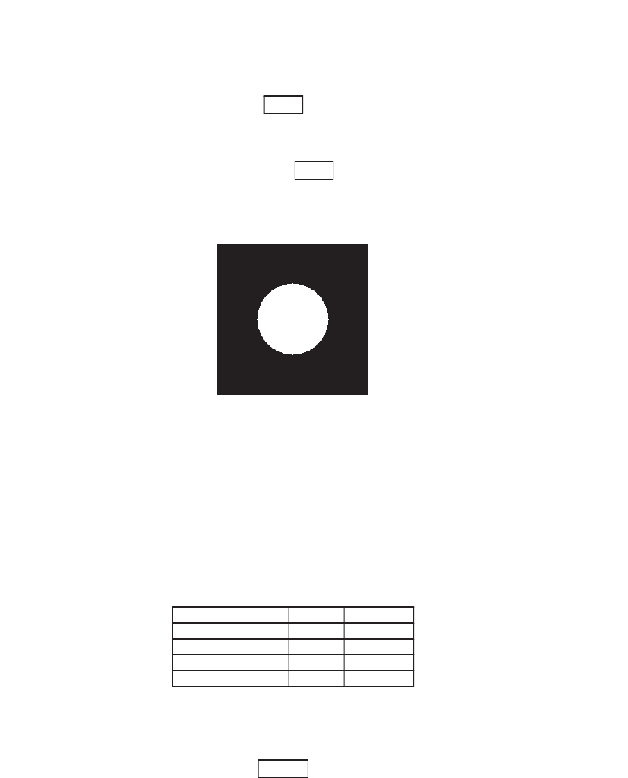
Marcellin et al. (2000) Zhang & F ritts (2004) . The 5/3 filter coefficients are listed in Table ??.
Analysis Coefficients Synthesis Coefficients
i h
o
(i) h
1
(i) h
o
(i) h
1
(i)
0 +
6
8
+1 +1 +
6
8
±1 +
2
8
−
1
2
−
1
2
+
2
8
±2 −
1
8
+
1
8
Table 1. Analysis and synthesis filter coefficients for the 5/3 wavele t.
Using the 5/3 integer wavelet, the highpass details d
j
(n) can be compute d using a lifting
based approach:
d
j
(n)=c
j+1
(2n + 1) −
c
j+1
(2n)+c
j+1
(2n + 2)
2
, (39)
where
�X� is the greatest integer less than or equal to X. The lo w frequency, average
coefficients c
j
(n) may be found using an update function
c
j
(n)=c
j+1
(2n)+
d
j
(n)+d
j
(n −1)+2
4
. (40)
For reconstruction, the reverse DWT can be found by reversing the arithmetic operations of
the forward transform. This is shown below:
c
j+1
(2n)=c
j
(n)+
d
j
(n)+d
j
(n −1)+2
4
, (41)
c
j+1
(2n + 1)=d
j
(n) −
c
j+1
(2n)+c
j+1
(2n + 2)
2
. (42)
These equations may be appli ed separably to the images in order to gain a 2-D DWT
representation.
5. Shift-invariant discr ete wavelet transform
Although the DWT is scale-invariant, it is well known that the DWT is shift-variant Mallat
(1998), i.e. the coefficients of a circularly shifted image are not transl ated versions of the
197
Shift-Invariant DWT for Medical Image Classification
original image’s coefficients. F or instance, the DWT of an input biomedical image f (x, y)
can be shown as:
f
(x, y) −→ DWT −→
F
(k
1
, k
2
, j)
where
F(k
1
, k
2
, j) are the 2-D DWT coefficients at scale j. A shift of the image will result in a
different set of coefficients
f
(x + Δx, y + Δy) −→ DWT −→
F
(k
�
1
, k
�
2
, j)
where k
�
1
�= k
1
+ a
1
·Δx and k
�
2
�= k
2
+ a
2
·Δy for (a
1
, a
2
), (Δx, Δy) ∈ Z, indicating that the two
sets of coefficients are not translated versions of one another.
Shift-variance causes significant chall enges in a feature extraction problem. For example,
Fig. 12. Image (simulated benign lesion).
consider the image of Figure 12 (the ce nter circle can be considered as a circumscribed benign
lesion, or something to that effect). If this circle is translated by a small amount ( which is
equivalent to the lesion being located in different regions of an image), the extracted features
would be different. To illustrate this, the image in Figure 12 is translated by shifts of
(Δx, Δy)
= {(0,0), (0,1), (1,0), (1,1)} and for each translation, the DWT is performed. Then, the mean
and variance of the wavelet coefficients are extracted from the LH band (moments are RST
invariant, so any invariance would be a conseq uence of the transform). The e xtracted features
are shown in Table 2. As shown by these resul ts, images with pathology (tex ture) located
in different regions of the images would result in different feature sets, thus leading to high
misclassification results.
For shift-invariant features, it is necessary to utilize a shift-invariant discrete wavelet
Input shift (Δx, Δy) Mean μ Variance σ
2
(0,0) -0.050537 97.017
(0,1) -0.051025 100.42
(1,0) 0.057861 96.82
(1,1) 0.058350 98.383
Table 2. Mean μ and variance σ
2
of the DWT coefficients of the LH band for circular
transl ates
(Δx, Δy) of Figure 12.
transform (SIDWT) on the input image f
(x, y)
f (x, y) −→ SIDWT −→
F
(k
1
, k
2
, j)
198
Discrete Wavelet Transforms - Theory and Applications