Olkkonen J. (ed.) Discrete Wavelet Transforms - Theory and Applications
Подождите немного. Документ загружается.

Part 1
Non-stationary Signals

0
Discrete Wavelet Analyses for Time Series
José S. Murguía and Haret C. Rosu
UASLP, IPICYT
México
1. Introduction
One frequent way of collecting experimental data by scientists and engineers is as sequences
of values at regularly spaced intervals in time. These sequences are called time-series. The
fundamental problem with the d ata in the form of time-series is how to process them in order
to ex tract meaningful and correct information, i.e., the possible signals embedded in them.
If a time-series i s stationary one can think that it can have harmonic compo nents that can
be detected by means of Fourier analysis, i.e., Fourier transforms (FT). However, in recent
times, it became evident that many time-seri es are not s tationary in the sense that their mean
properties change in time. The waves of infinite support that f orm the har monic components
are not adequate i n the latter case in which one needs waves localized not only in freq uency
but in time as well. They have been called wavelets and allow a time-scale decomposition of a
sig nal. Significant progress in under standing the wavelet process ing of non-stationary signals
has been achieved over the last two decades. However, to get the dynamics that produces a
non-stationary signal it is crucial that in the corresponding time-ser ies a correct separation
of the fluctuations from the average behavior, or trend, is performed. Therefore, people had
to invent novel statisti cal methods of detrending the data that should be com b ined with the
wavelet analysis. A bunch of such techniques have been developed lately for the important
class of non-stationary time series that di splay multi-scaling behavior of the multi-fractal
type. Our goal in this chapter is to present our experience with the wavelet processi ng,
based mainly on the discrete wavelet transform (DWT), of non-statio nary fractal time-series
of elementary cel lular automata and the non-stationary chaotic time-series produced by a
three-state non-linear ele ctronic circuit.
2. The wavelet transform
Let L
2
(R) denote the space of all square integrable functions on R. In signal processing
parlance, it is the space of functions with finite energy. Let ψ
(t) ∈ L
2
(R) be a fixed function.
The function ψ
(t) is said to be a wavelet if and only if its FT
ˆ
ψ(ω) satisfies
C
ψ
=
∞
0
|
ˆ
ψ
(ω)|
2
|ω|
dω < ∞. (1)
The relation (1) is called the admissibility condition (Daubechies, 1992; Mallat, 1999; Strang,
1996; Qian, 2002), which implies that the wavelet must have a zero average
∞
−∞
ψ(t)dt =
ˆ
ψ
(0)=0, (2)
0
Discrete Wavelet Analyses for Time Series
José S. Murguía and Haret C. Rosu
UASLP, IPICYT
México
1. Introduction
One frequent way of collecting experimental data by scientists and engineers is as sequences
of values at regularly spaced intervals in time. These sequences are called time-series. The
fundamental problem with the d ata in the form of time-series is how to process them in order
to ex tract meaningful and correct information, i.e., the possible signals embedded in them.
If a time-series i s stationary one can think that it can have harmonic compo nents that can
be detected by means of Fourier analysis, i.e., Fourier transforms (FT). However, in recent
times, it became evident that many time-seri es are not s tationary in the sense that their mean
properties change in time. The waves of infinite support that f orm the har monic components
are not adequate i n the latter case in which one needs waves localized not only in freq uency
but in time as well. They have been called wavelets and allow a time-scale decomposition of a
sig nal. Significant progress in under standing the wavelet process ing of non-stationary signals
has been achieved over the last two decades. However, to get the dynamics that produces a
non-stationary signal it is crucial that in the corresponding time-ser ies a correct separation
of the fluctuations from the average behavior, or trend, is performed. Therefore, people had
to invent novel statisti cal methods of detrending the data that should be com b ined with the
wavelet analysis. A bunch of such techniques have been developed lately for the important
class of non-stationary time series that di splay multi-scaling behavior of the multi-fractal
type. Our goal in this chapter is to present our experience with the wavelet processi ng,
based mainly on the discrete wavelet transform (DWT), of non-statio nary fractal time-series
of elementary cel lular automata and the non-stationary chaotic time-series produced by a
three-state non-linear ele ctronic circuit.
2. The wavelet transform
Let L
2
(R) denote the space of all square integrable functions on R. In signal processing
parlance, it is the space of functions with finite energy. Let ψ
(t) ∈ L
2
(R) be a fixed function.
The function ψ
(t) is said to be a wavelet if and only if its FT
ˆ
ψ(ω) satisfies
C
ψ
=
∞
0
|
ˆ
ψ
(ω)|
2
|ω|
dω < ∞. (1)
The relation (1) is called the admissibility condition (Daubechies, 1992; Mallat, 1999; Strang,
1996; Qian, 2002), which implies that the wavelet must have a zero average
∞
−∞
ψ(t)dt =
ˆ
ψ
(0)=0, (2)
1
Discrete Wavelet Analyses for Time Series
1
and therefore it must be oscillatory. In other words, ψ must be a sort of wave (Daubechies,
1992; Mallat, 1999).
Let us now define the dilated–translated wavelets ψ
a,b
as the following functions
ψ
a,b
(t)=
1
√
a
ψ
t
−b
a
, (3)
where b
∈ R is a translation parameter, whereas a ∈ R
+
(a �= 0) is a dilation or scale
parameter. T he factor a
−1/2
is a normalization constant such that the energy, i.e., the v alue
provided through the square integrability of ψ
a,b
, is the same for all scales a. One notices that
the scale parameter a in (3) rules the dilations of the independent variable
(t − b). In the same
way, the factor a
−1/2
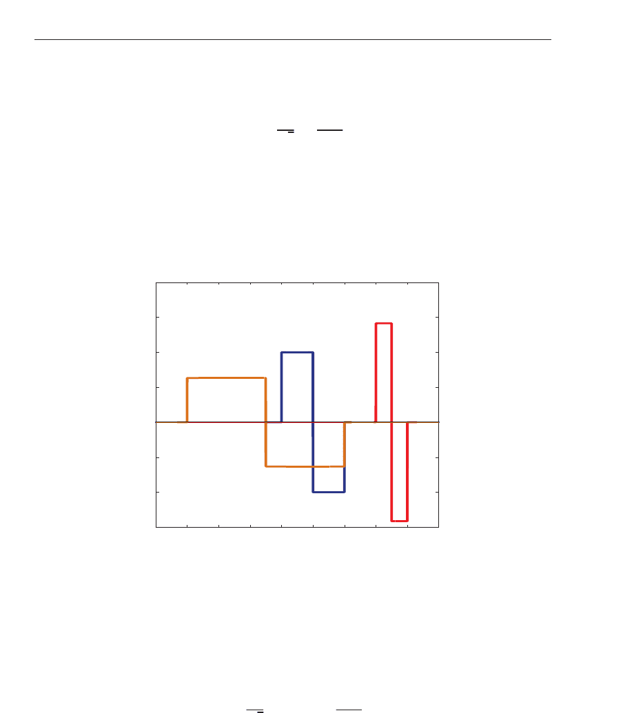
rules the dilation in the values taken by ψ, se e the y-axis in Fig. 1. With (3),
one is able to decompose a square integrable function x
(t) in terms of these dilated –translated
wavelets.
−2 −1.5 −1 −0.5 0 0.5 1 1.5 2 2.5
−1.5
−1
−0.5
0
0.5
1
1.5
2
ψ
a, b
(t)
t
ψ
5/2, −3/2
(t)
ψ
1/2, 3/2
(t)
ψ
1, 0
(t)
Fig. 1. The Haar wavelet function for se veral value s of the scale parameter a and translation
parameter b. If a
< 1, the wavelet functi on is contracted, and if a > 1, the wavelet is
expanded.
The continuous wavelet transform (CWT) of x
(t) ∈ L
2
(R) is defined as
W
x
(a, b)=�x, ψ
a,b
� =
∞
−∞
x(t)
¯
ψ
a,b
(t)dt
=
1
√
a
∞
−∞
x(t)
¯
ψ
t
−b
a
dt, (4)
where
� , � is the scalar product in L
2
(R) defined as �f , g� :=
f (t)
¯
g
(t)dt, and the symbol “¯”
denotes complex co njugation. The CWT (4) measures the variation of x in a neighborhood of
the point b, whose size is proportional to a.
4
Discrete Wavelet Transforms - Theory and Applications

and therefore it must be oscillatory. In other words, ψ must be a sort of wave (Daubechies,
1992; Mallat, 1999).
Let us now define the dilated–translated wavelets ψ
a,b
as the following functions
ψ
a,b
(t)=
1
√
a
ψ
t
−b
a
, (3)
where b
∈ R is a translation parameter, whereas a ∈ R
+
(a �= 0) is a dilation or scale
parameter. T he factor a
−1/2
is a normalization constant such that the energy, i.e., the v alue
provided through the square integrability of ψ
a,b
, is the same for all scales a. One notices that
the scale parameter a in (3) rules the dilations of the independent variable
(t − b). In the same
way, the factor a
−1/2
rules the dilation in the values taken by ψ, se e the y-axis in Fig. 1. With (3),
one is able to decompose a square integrable function x
(t) in terms of these dilated –translated
wavelets.
−2 −1.5 −1 −0.5 0 0.5 1 1.5 2 2.5
−1.5
−1
−0.5
0
0.5
1
1.5
2
ψ
a, b
(t)
t
ψ
5/2, −3/2
(t)
ψ
1/2, 3/2
(t)
ψ
1, 0
(t)
Fig. 1. The Haar wavelet function for se veral value s of the scale parameter a and translation
parameter b. If a
< 1, the wavelet functi on is contracted, and if a > 1, the wavelet is
expanded.
The continuous wavelet transform (CWT) of x
(t) ∈ L
2
(R) is defined as
W
x
(a, b)=�x, ψ
a,b
� =
∞
−∞
x(t)
¯
ψ
a,b
(t)dt
=
1
√
a
∞
−∞
x(t)
¯
ψ
t
−b
a
dt, (4)
where
� , � is the scalar product in L
2
(R) defined as �f , g� :=
f (t)
¯
g
(t)dt, and the symbol “¯”
denotes complex co njugation. The CWT (4) measures the variation of x in a neighborhood of
the point b, whose size is proportional to a.
If we are interested to reconstruct x from its wavelet transform (4) , we make use of the the
reconstruction formula, also called resolution of the identity (Daubechies, 1992; Mallat, 1999)
x
(t)=
1
C
ψ
∞
0
∞
−∞
W
x
(a, b)ψ
a,b
(t)
dadb
a
2
, (5)
where it is now clear why we imposed (1).
However, a huge amount of data are represented by a finite number of values, so it is
important to consider a discrete version of the CWT (4). Generally, the orthogonal(discrete)
wavelets are emplo yed because this method associates the wavelets to o rthonormal bases
of L
2
(R). In this case, the wavelet transform is performed only on a discrete grid of the
parameters of dilation and translation, i.e., a and b take only integral values. Within this
framework, an arbitrary signal x
(t) of finite ene rgy can be written using an orthonormal
wavelet basis:
x
(t)=
∑
m
∑
n
d
m
n
ψ
m
n
(t) , (6)
where the coefficients of the expansion are given by
d
m
n
=
∞
−∞
x(t)ψ
m
n
(t)dt . (7)
The orthonormal basi s functions are all dilations and translations of a function referred as the
analyzing wavelet ψ
(t) , and they can be expressed in the form
ψ
m
n
(t)=2
m/2
ψ(2
m
t − n), (8)
with m and n denoting the dilation and translation indices, respectively. The contribution of
the signal at a particular wavelet level m is given by
d
m
(t)=
∑
n
d
m
n
ψ
m
n
(t) , (9)
which pro vides infor mation on the time behavior of the signal within different scale bands.
Additionally, it provides knowledge of their contribution to the total signal energy.
In this context, Mallat (1999) developed a computationally efficient method to calculate (6) and
(7). This method is known as multiresolution analysis (MRA). The MRA approach provides
a general method for constructing orthogonal wavelet basis and l eads to the implementation
of the fast wavelet transform (FWT). This algorithm connects, in an elegant way, wavele ts
and filter banks. A multiresolution s ignal decomposition of a signal X is based on successive
decomposition into a series of approximations and details, which become increasingly coarse.
Associated with the wavelet function ψ
(t) is a corresponding scaling function, ϕ(t), and
scaling coefficients, a
m
n
(Mallat, 1999). The scaling and wavel et coefficients at scale m can be
computed from the scaling coefficients at the next finer scale m
+ 1 using
a
m
n
=
∑
l
h[l −2n]a
m+1
l
, (10)
d
m
n
=
∑
l
g[l − 2n]a
m+1
l
, (11)
where h
[n] and g[n] are typically called lowpass and highpass filters in the associated filter
bank. Equations (10) and (11) represent the fast wavelet trans form (FWT) for computing (7). In
5
Discrete Wavelet Analyses for Time Series
fact, the signals a
m
n
and d
m
n
are the convolutions of a
m+1
n
with the filters h[n] and g[n] followed
by a downsam pling o f factor 2 (Mallat, 1999).
Conversely, a reconstruction of the original scaling coe fficients a
m+1
n
can be made from
a
m+1
n
=
∑
l
(
h[2l − n]a
m
l
+ g[2l − n]d
m
l
)
, (12)
a combination of the scaling and wavelet coefficients at a coarse scale. Equation (12) represents
the inverse of FWT for computing (6), and it corresponds to the synthesi s filter bank. This part
can be viewed as the discrete convol utions between the upsampled signal a
m
l
and the filters
h
[n] and g[n], that is, following an “upsampling” of factor 2 one calculates the convo lutions
between the upsampl ed signal and the filter s h
[n] and g[n]. The number of levels in the
multiresolution algorithm depends on the length of the signal. A signal with 2
k
values can
be decomposed into k
+ 1 levels. To initialize the FWT, one considers a discrete time signal
X
= {x[1], x[2],.. .,x[N]} of length N = 2
M
. The first application of (10) and (11), beg inning
with a
m+1
n
= x[n], defi nes the first level of the FWT of X. The process goes on, always adopting
the “m
+ 1” scaling coefficients to calculate the “m” scaling and wavelet coefficients. Iterating
(10) and (11) M times, the transform ed signal consis ts of M sets of wavelet coefficients at
scales m
= 1,...,M, and a signal set of scaling coefficients at scale M. There are exactly 2
(k−m)
wavelet coefficients d
m
n
at each scale m,and2
(k−M)
scaling coefficients a
M
n
. The maximum
number of iterations M
max
is k. This property of the MRA is generally the key factor to identify
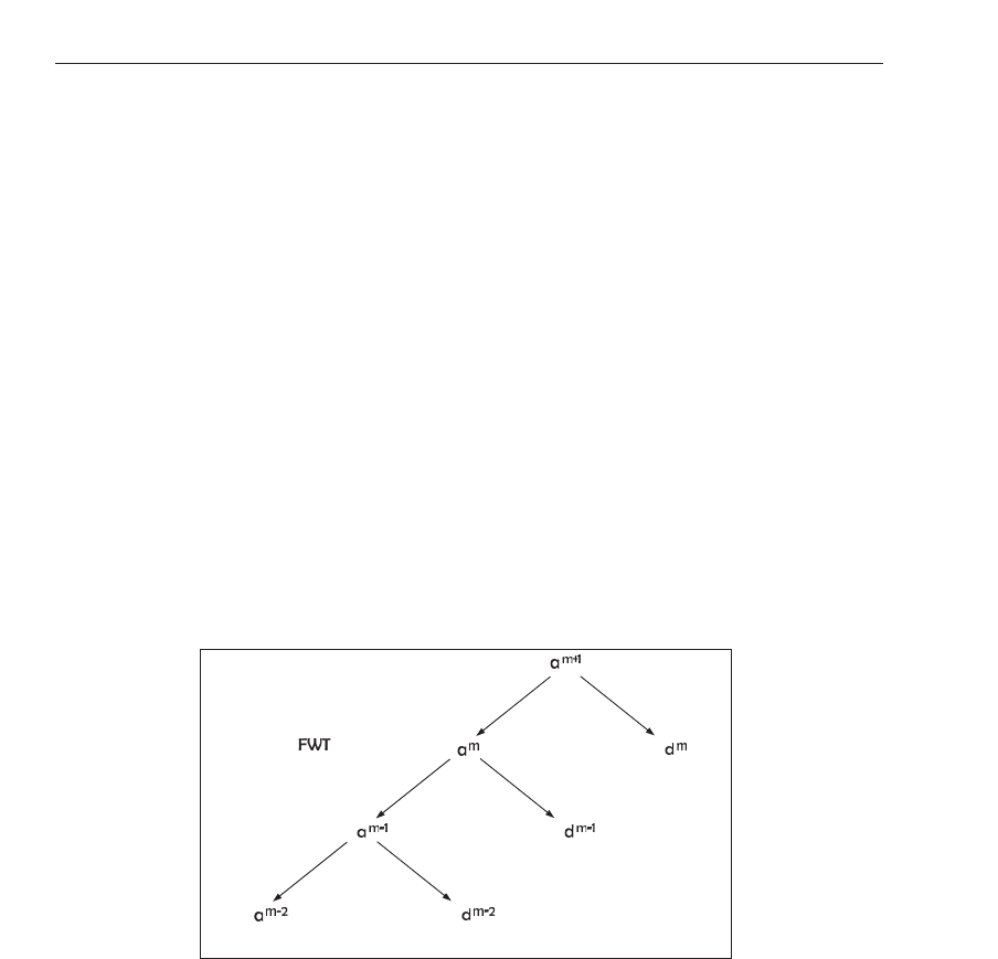
crucial information in the respective frequency bands. A three-level decomposition process of
the FWT is shown in Fig. 2.
Fig. 2. The structure of a three-level fast wavelet transfo rm.
In a broad sense, with this approach, the low-pass coefficients capture the trend and the
high-pass coefficients keep track of the fluctuations in the data. The scali ng and wavelet
functions are natur ally endowed with an app ropriate window size, which manifests in the
scale index or level, and hence they can capture the local averages and differences, in a
window of one’s choice.
When someone is interested to measure the local or global regularity of a signal, some
degree of regularity is useful in the wavelet basis for the representation to be well behaved
(Daubechies, 1992; Mallat, 1999). To achieve this, a wavelet function should have n vanishing
moments. A wavelet is said to have n vanishing moments if and only if it satisfies
∞
−∞
t
k
ψ(t)dt = 0 for k = 0,1,...,n − 1 and
∞
−∞
t
k
ψ(t)dt �= 0 for k = n. This m eans that
6
Discrete Wavelet Transforms - Theory and Applications
fact, the signals a
m
n
and d
m
n
are the convolutions of a
m+1
n
with the filters h[n] and g[n] followed
by a downsam pling o f factor 2 (Mallat, 1999).
Conversely, a reconstruction of the original scaling coe fficients a
m+1
n
can be made from
a
m+1
n
=
∑
l
(
h[2l − n]a
m
l
+ g[2l − n]d
m
l
)
, (12)
a combination of the scaling and wavelet coefficients at a coarse scale. Equation (12) represents
the inverse of FWT for computing (6), and it corresponds to the synthesi s filter bank. This part
can be viewed as the discrete convol utions between the upsampled signal a
m
l
and the filters
h
[n] and g[n], that is, following an “upsampling” of factor 2 one calculates the convolutions
between the upsampl ed signal and the filter s h
[n] and g[n]. The number of levels in the
multiresolution algorithm depends on the length of the signal. A signal with 2
k
values can
be decomposed into k
+ 1 levels. To initialize the FWT, one considers a discrete time signal
X
= {x[1], x[2],.. .,x[N]} of length N = 2
M
. The first application of (10) and (11), beg inning
with a
m+1
n
= x[n], defi nes the first level of the FWT of X. The process goes on, always adopting
the “m
+ 1” scaling coefficients to calculate the “m” scaling and wavelet coefficients. Iterating
(10) and (11) M times, the transform ed signal consis ts of M sets of wavelet coefficients at
scales m
= 1,...,M, and a signal set of scaling coefficients at scale M. There are exactly 2
(k−m)
wavelet coefficients d
m
n
at each scale m,and2
(k−M)
scaling coefficients a
M
n
. The maximum
number of iterations M
max
is k. This property of the MRA is generally the key factor to identify
crucial information in the respective frequency bands. A three-level decomposition process of
the FWT is shown in Fig. 2.
Fig. 2. The structure of a three-level fast wavelet transfo rm.
In a broad sense, with this approach, the low-pass coefficients capture the trend and the
high-pass coefficients keep track of the fluctuations in the data. The scali ng and wavelet
functions are natur ally endowed with an app ropriate window size, which manifests in the
scale index or level, and hence they can capture the local averages and differences, in a
window of one’s choice.
When someone is interested to measure the local or global regularity of a s ignal, some
degree of regularity is useful in the wavelet basis for the representation to be well behaved
(Daubechies, 1992; Mallat, 1999). To achieve this, a wavelet function should have n vanishing
moments. A wavelet is said to have n vanishing moments if and only if it satisfies
∞
−∞
t
k
ψ(t)dt = 0 for k = 0,1,...,n − 1 and
∞
−∞
t
k
ψ(t)dt �= 0 for k = n. This m eans that
a wavelet with n vanishing moments is orthogonal to all polynomials up to order n −1. Thus,
the DWT of x
(t) performed with a wavelet ψ( t) with n vanishing moments is nothing else
but a “smoothed version” of the n
−th derivative of x(t) on various scales. This important
property helps detrending the data.
In addition, another important property is that the total energy of the signal may be expressed
as follows
N
∑
n=1
|x[n]|
2
=
N
∑
n=1
|a
M
n
|
2
+
M
∑
m=1
N
∑
n=1
|d
m
n
|
2
. (13)
This can be identified as Parseval’s relation in terms of wavelets, where the signal
energy can be calculated in terms of the different resolution levels of the corresponding
wavelet-transformed signal. A more detailed treatment of this subject can be found in ( Mallat,
1999).
3. Multifractal analysis of cellular automata time series
3.1 Cellular automata
An elementary cellular automaton(ECA) can be considered as a discrete dynamical that evolve
at discrete time steps. An ECA is a cellular automata consisting of a chain o f N lattice sites with
each site is denoted by an index i. Associated with each site i is a dynamical variable x
i
which
can take only k discrete values. Most of the studies have been done with k
= 2, where x
i
= 0 or
1. Therefore there are 2
N
different states for these automata. One can se e that the time, space,
and states of this system take only discrete values. The ECA considered evolves according to
the local rule
x
t+1
n
=[x
t
n
−1
+ x
t
n
+1
]mod 2 , (14)
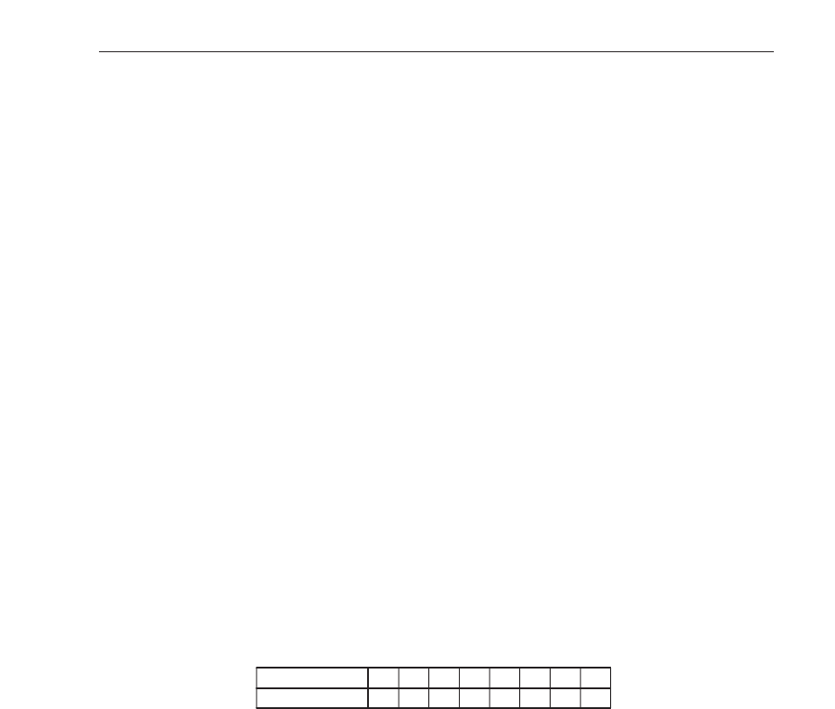
which corresponds to the rule 90. Table 1 is the lookup table of this ECA rule, where it
is s pecified the evolution from the neighborhood configu ration ( first row) to the next state
(second row), that is, the next state of i
−th cell depends on the present states of its left and
right neighbors.
Neighborhood 111 110 101 100 011 010 001 000
Rule result 0 1 0 1 1 0 1 0
Table 1. Elementary rule 90. The second row shows the future state of the cell if it and its
neighbors are in the arrangement shown above in the first row.
In fact, a rule is numbered by the unsigned decimal equivalent of the binary expression in
the second row. When the same rule is applied to update cells of ECA, such ECA are called
uniform ECA; otherwise the ECA are called non-uniform or hybrids. It is important to observe
that the evolution rules of ECA are d etermined by two main factors, the rule and the initial
conditions.
3.2 WMF-DFA algorithm
To reveal the MF properties (Halsey e t al., 1986) of ECA, we follow a variant of the M F-DFA
with the discrete wavelet method proposed in (Manimaran e t al., 2005). This algorithm will
separate the trends from fluctuations, in the ECA time series, using the fact that the low-pass
version resembles the original data in an “averaged” manner in different resolutions. Instead
7
Discrete Wavelet Analyses for Time Series

of a polynomial fit, we consider the different versions of the low-pass coefficients to calculate
the “local” trend. This method involves the following steps.
Let x
(t
k
) be a time series type of data, where t
k
= kΔt and k = 1,2,..., N.
1. Determine the profile Y
(k)=
∑
k
i
=1
(x(t
i
) −�x�) of the time series, which is the cumulative
sum of the series from which the series mean value is subtr acted.
2. Compute the fast wavelet transform (FWT), i.e., the multilevel wavelet decomposition of
the profile. For each level m, we get the fluctuations of the Y
(k) by subtracting the “local”
trend of the Y data, i.e., ΔY
(k; m)=Y(k) −
˜
Y
(k; m), whe re
˜
Y(k; m) is the reconstructed
profile after removal of successive details coefficients at each level m. These fluctuations at
level m are subdivided into windows, i.e., into M
s
= int(N/s) non-overlapping segments
of length s. This division is performed starting from both the beginning and the end of
the fluctuations series (i.e., one has 2M
s
segments). Next, one calculates the l ocal variances
associated to each window ν
F
2
(ν, s; m)=var
[
ΔY((ν − 1)s + j; m)
]
, j = 1, ..., s , ν = 1, ..., 2M
s
, M
s
= int(N/s) . (15)
3. Calculate a q
−th order fluctuation function defined as
F
q
(s; m)=
1
2M
s
2M
s
∑
ν=1
|F
2
(ν, s; m)|
q /2
1/q
(16)
where q
∈ Z with q �= 0. Because of the diverging exponent when q → 0 we employed
in this limit a logarithmic averaging F
0
(s; m)=exp
1
2M
s
2M
s
∑
ν=1
ln |F
2
(ν, s; m)|
as in
(Kantelhardt et al., 2002; Telesca et al., 2004).
To determine if the analyzed time series have a fractal scaling behavior, the fluctuation
function F
q
(s; m) should reveal a power law scaling
F
q
(s; m) ∼ s
h(q)
, (17)
where h
(q) is called the generalized Hurst exponent (Telesca et al., 2004) since it can depend
on q, while the original Hurst exponent is h
(2). If h is constant for al l q then the time
ser ies is monofractal, otherwise it has a M F behavior. In the latter case, one can calculate
various other MF scaling exponents, such as τ
(q)=qh(q) − 1 and f (α) (Halsey et al.,
1986). A linear behavior of τ
(q) indicates monofractality whereas the non-linear behavior
indicates a multifr actal signal. A fundamental result in the multifractal formalism states that
the singularity spectrum f
(α) is the Legendre transform of τ(q), i.e.,
α
= τ
�
(q), and f (α)=qα − τ(q).
The singularity spectrum f
(α) is a non- negative convex function that is supported on the
closed interval
[α
min
, α
max
]. In fact, the strength of the multifractality is roughly me asured
with the width Δα
= α
max
− α
min
of the parabolic singularity spectrum f (α) on the α axis,
where the boundary values of the support, α
min
for q > 0 and α
max
for q < 0, correspond to
the strongest and weakest singularity, respec tively.
8
Discrete Wavelet Transforms - Theory and Applications