Olkkonen J. (ed.) Discrete Wavelet Transforms - Theory and Applications
Подождите немного. Документ загружается.

of a polynomial fit, we consider the different versions of the low-pass coefficients to calculate
the “local” trend. This method involves the following steps.
Let x
(t
k
) be a time series type of data, where t
k
= kΔt and k = 1,2,..., N.
1. Determine the profile Y
(k)=
∑
k
i
=1
(x(t
i
) −�x�) of the time series, which is the cumulative
sum of the series from which the serie s mean value is subtr acted.
2. Compute the fast wavelet transform (FWT), i.e., the multilevel wavelet decomposition of
the profile. For each level m, we get the fluctuations of the Y
(k) by subtracting the “local”
trend of the Y data, i.e., ΔY
(k; m)=Y(k) −
˜
Y
(k; m), whe re
˜
Y(k; m) is the reconstructed
profile after removal of successive details coefficients at each level m. These fluctuations at
level m are subdivided into windows, i.e., into M
s
= int(N/s) non-overlapping segments
of length s. This division is performed starting from both the beginning and the end of
the fluctuations series (i.e., one has 2M
s
segments). Next, one calculates the l ocal variances
associated to each window ν
F
2
(ν, s; m)=var
[
ΔY((ν − 1)s + j; m)
]
, j = 1, ..., s , ν = 1, ..., 2M
s
, M
s
= int(N/s) . (15)
3. Calculate a q
−th order fluctuation function defined as
F
q
(s; m)=
1
2M
s
2M
s
∑
ν=1
|F
2
(ν, s; m)|
q /2
1/q
(16)
where q
∈ Z with q �= 0. Because of the diverging exponent when q → 0 we employed
in this limit a logarithmic averaging F
0
(s; m)=exp
1
2M
s
2M
s
∑
ν=1
ln |F
2
(ν, s; m)|
as in
(Kantelhardt et al., 2002; Telesca et al., 2004).
To determine if the analyzed time series have a fractal scaling behavior, the fluctuation
function F
q
(s; m) should reveal a power law scaling
F
q
(s; m) ∼ s
h(q)
, (17)
where h
(q) is called the generalized Hurst exponent (Telesca et al., 2004) since it can depend
on q, while the original Hurst exponent is h
(2). If h is constant for al l q then the time
ser ies is monofractal, otherwise it has a M F behavior. In the latter case, one can calculate
various other MF scaling exponents, such as τ
(q)=qh(q) − 1 and f (α) (Halsey et al.,
1986). A linear behavior of τ
(q) indicates monofractality whereas the non-linear behavior
indicates a multifr actal signal. A fundamental result in the multifractal formalism states that
the singularity spectrum f
(α) is the Legendre transform of τ(q), i.e.,
α
= τ
�
(q), and f (α)=qα − τ(q).
The singularity spectrum f
(α) is a non- negative convex function that is supported on the
closed interval
[α
min
, α
max
]. In fact, the strength of the multifractality is roughly me asured
with the width Δα
= α
max
− α
min
of the parabolic singularity spectrum f (α) on the α axis,
where the boundary values of the support, α
min
for q > 0 and α
max
for q < 0, correspond to
the strongest and weakest singularity, respectively.
3.3 Application of WMF- DFA
To illustrate the efficiency of the wavelet multifractal procedure, we first carry out the analysis
of the binomial multifractal model (Fe der, 1998; Kantelhardt et al., 2002).
For the multifractal time series generated through the binomial multi fractal model , a series
of N
= 2
n
max
numbers x
k
, with k = 1,...,N, is defined by
x
k
= a
n(k−1)
(1 − a)
n
max
−n(k−1)
. (18)
where 0.5
< a < 1 is a parameter and n(k) is the number of digits equal to 1 in the binary
representation of the index k. The scaling exponent h
(q) and τ(q) can be calculated e xactly in
this model. These exponents have the closed form
h
(q)=
1
q
−
ln[a
q
+(1 − a )
q
]
q ln 2
, τ
(q)=−
ln[a
q
+(1 − a )
q
]
ln 2
. (19)
In Table 2 and Fig. 3, we present the comp arison of the multifractal quantity h for a
= 2/3
between the values for the theoretical case (h
T
(q)), with the numerical results obtained
through wavelet analysis (h
W
(q)). Notice that the numerical valu es have a slight downward
transl ation. Adding a vertical offset (Δ
= h
T
(1) − h
W
(1)) to h
W
(q), we can notice that both
values theoretically and numerically are very close.
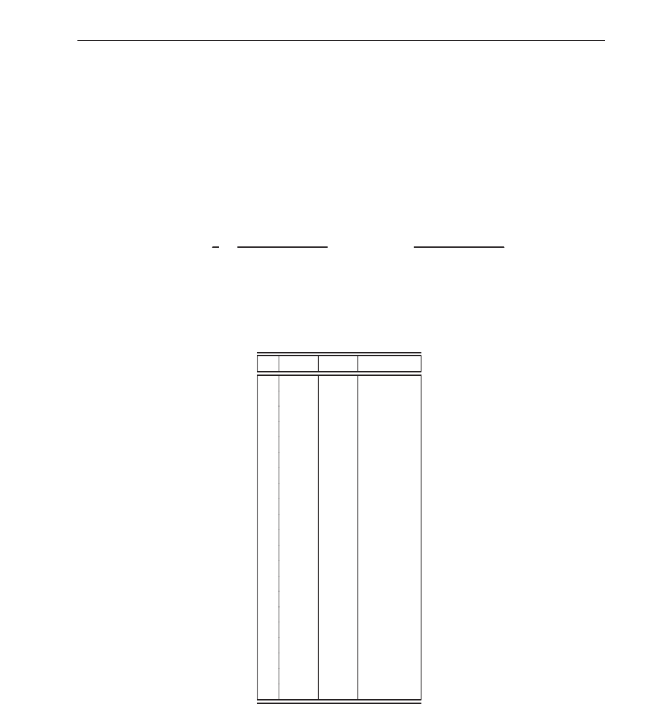
q h
T
(q) h
W
(q) h
W
(q)+Δ
-10 1.4851 1.4601 1.4851
-9 1.4742 1.4498 1.4749
-8 1.4607 1.4373 1.4623
-7 1.4437 1.4217 1.4467
-6 1.4220 1.4018 1.4269
-5 1.3938 1.3761 1.4012
-4 1.3568 1.3422 1.3673
-3 1.3083 1.2971 1.3221
-2 1.2459 1.2376 1.2627
-1 1.1699 1.1626 1.1876
0 0.0000 1.0742 1.0992
1 1.0000 0.9809 1.0059
2 0.9240 0.8961 0.9212
3 0.8617 0.8286 0.8537
4 0.8131 0.7780 0.8031
5 0.7761 0.7401 0.7652
6 0.7479 0.7112 0.7362
7 0.7262 0.6887 0.7137
8 0.7093 0.6711 0.6961
9 0.6958 0.6570 0.6821
10 0.6848 0.6457 0.6707
Table 2. The values of the generalized Hurst exponent h for the binomial multifractal model
with a
= 2/3, which were computed analytically and with the wavelet approach.
In a similar way, we analyze the time series of the so-called row sum ECA signals, i.e., the sum
of ones in sequences of rows, employing the db-4 wavelet function, another wavelet function
that belongs to the Daubechies family (Daubechies, 1992; Mal lat, 1999). We have found that
9
Discrete Wavelet Analyses for Time Series
0 2 4 6 8 10 12 14 16 18 20 22
0
0.2
0.4
0.6
0.8
1
1.2
1.4
1.6
q
h(q)
Theoretical
WMF−DFA
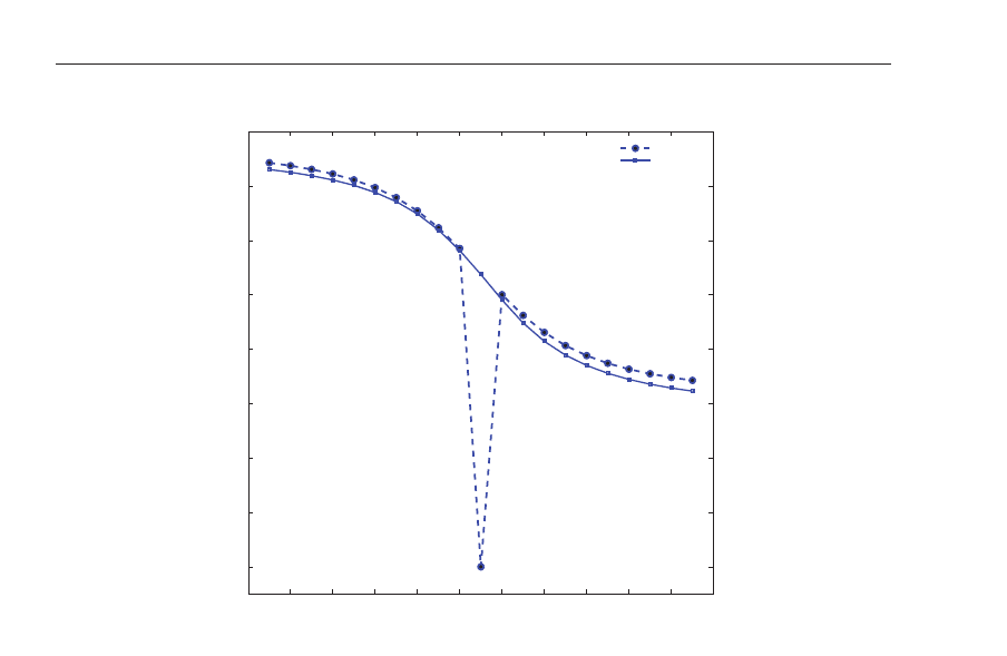
Fig. 3. The generalized Hurst exponent h for the binomial multifractal model with a = 2/3.
The theoretical values of h
(q) with the WMF-DFA calculations are shown for comparison.
a better matching of the results given by the WMF-DFA me thod with those of other metho ds
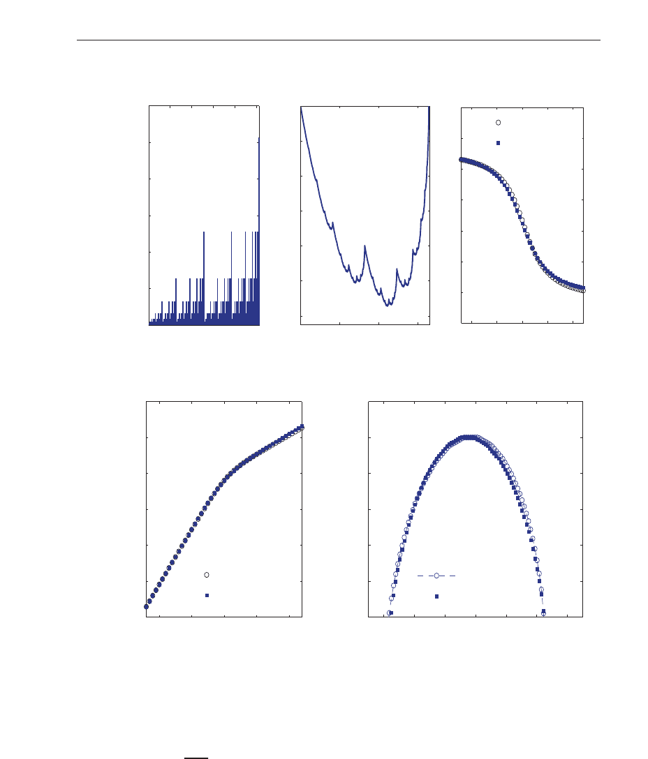
is provided with this wavelet function. Figure 4 illustrates the results for the rule 90, when
the first row is all 0s with a 1 in the center, i.e., the impulsive initial condition. The fact that
the generalized Hurst exponent is not a constant horizontal line is indicative of a multifractal
behavior in this ECA time series. In addition, if the τ index is not of a single slope, it can be
considered as another clear feature of multifractality.
For the impulsive initial condition in ECA rule 90 the most “frequent” singularity for the
analyzed time series occurs at α
= 0.568, and Δα = 1.0132(0.9998) when the WMF-DFA
(MF-DFA) are employed. Reference (Murguía et al., 2009) presents the results for different
initial center pulses fo r rules 90, 105, and 150, where the width Δα of rule 90 is shifted to the
right with res pect to those of 105 and 150. In addition, the strongest singul arity, α
min
, of all
these time seri es corresponds to the rule 90 and the weakes t singularity, α
max
, to the rule 150.
With the aim of computing the pseudo-random sequences of N bits, in Reference (Mejía
& Urías, 2001) an algorithm based on the backward evolution of the CA rule 90 has
been proposed. A modification of the generator producing pseudo-random sequences has
been recently consi dered in (Murguía et al., 2010). The latter pro posal is i mplemented and
studied in terms of the sequence matrix H
N
, which was used to generate recursively the
pseudo-random sequences.
This matrix has dimensions
(2N + 1) × (2N + 1). Since the evolution of the sequence matrix
H
N
is based on the evolution of the ECA rule 90, the structure of the patterns of bits of the
latter must be directly reflected in the structure of the entries of H
N
.
10
Discrete Wavelet Transforms - Theory and Applications
0 2 4 6 8 10 12 14 16 18 20 22
0
0.2
0.4
0.6
0.8
1
1.2
1.4
1.6
q
h(q)
Theoretical
WMF−DFA
Fig. 3. The generalized Hurst exponent h for the binomial multifractal model with a = 2/3.
The theoretical values of h
(q) with the WMF-DFA calculations are shown for comparison.
a better matching of the results given by the WMF-DFA method with those of other metho ds
is provided with this wavelet function. Figure 4 illustrates the results for the rule 90, when
the first row is all 0s with a 1 in the center, i.e., the impulsive initial condition. The fact that
the generalized Hurst exponent is not a constant horizontal line is indicative of a multifractal
behavior in this ECA time series. In addition, if the τ index is not of a single slope, it can be
considered as another clear feature of multifractality.
For the impulsive initial condition in ECA rule 90 the most “frequent” singularity for the
analyzed time series occurs at α
= 0.568, and Δα = 1.0132(0.9998) when the WMF-DFA
(MF-DFA) are employed. Reference (Murguía et al., 2009) presents the results for different
initial center pulses fo r rules 90, 105, and 150, where the width Δα of rule 90 is shifted to the
right with res pect to those of 105 and 150. In addition, the strongest singul arity, α
min
, of all
these time seri es corresponds to the rule 90 and the weakes t singularity, α
max
, to the rule 150.
With the aim of computing the pseudo-random sequences of N bits, in Reference (Mejía
& Urías, 2001) an algorithm based on the backward evolution of the CA rule 90 has
been proposed. A modification of the generator producing pseudo-random sequences has
been recently consi dered in (Murguía et al., 2010). The latter pro posal is i mplemented and
studied in terms of the sequence matrix H
N
, which was used to generate recursively the
pseudo-random sequences.
This matrix has dimensions
(2N + 1) × (2N + 1). Since the evolution of the sequence matrix
H
N
is based on the evolution of the ECA rule 90, the structure of the patterns of bits of the
latter must be directly reflected in the structure of the entries of H
N
.
50 100 150 200 250
0
50
100
150
200
250
300
(a)
n
x
0 5000 10000 15000
−12
−10
−8
−6
−4
−2
0
x 10
5
(b)
n
Y
−10 −5 0 5 10
0.4
0.6
0.8
1
1.2
1.4
1.6
(c)
q
h(q)
−10 −5 0 5 10
−20
−15
−10
−5
0
5
10
(d)
q
τ(q)
0 0.2 0.4 0.6 0.8 1 1.2
0
0.2
0.4
0.6
0.8
1
(e)
α
f(α)
WMF−DFA
MFDFA
WMF−DFA
MFDFA
WMF−DFA
MFDFA
Fig. 4. (a) Time series of the row signal of the cellular automata rule 90. Only the first 2
8
points are shown of the whole set of 2
14
data points. Profile Y of the row signal. (d)
Generalized Hurst exponent h
(q). (e) The τ exponent, τ(q)=qh(q) − 1. (f) The singularity
spectrum f
(α)=q
dτ(q)
dq
−τ(q). The calculations of the multifractal q uantities h, τ , and f (α)
are per formed both with the MF-DFA and the wavelet-based WMF-DFA.
11
Discrete Wavelet Analyses for Time Series

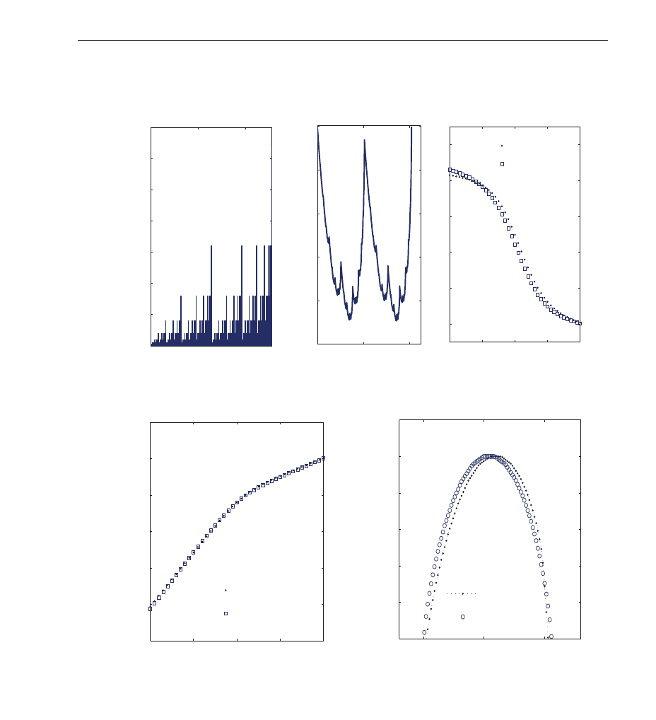
Here, in the same spirit as in Ref. (Murguía et al ., 2009), we also analyze the sum of ones in
the sequences of the rows of the matrix H
N
with the db-4 wavelet function. The results for the
row sums of H
2047
are illustrated in Fig. 5, through which we confirm the multifractality of
this time series. The width Δα
H
2047
= 1.12 −0.145 = 0.975, and the most “frequent” singularity
occurs at α
mf
H
2047
= 0.638. Although the profile is different, the results are similar with those
obtained for the rule 90 with a slight shifting, see Fig. 4. A more complete analysis of this
matrix is car ried out in (Murguía et al., 2010).
4. Chaotic time series
In this section, we study the dynamics of experimental time series generated by an electronic
chaotic circuit. The wavelet analysis of these experimental chaotic time s eries gives us useful
information of such system through the energy concentration at specific wavelet levels.
It is known that the wavelet variance provides a very efficient measure of the structure
contained within a time series because of the ability of wavelet transforms to allot small
wavelet coeffici ents to the s moother par ts of a signal in contrast with the sharp, non-stationary
behavior which gives rise to local maxima (see, for example, Chapter 8 in the book of Percival
and Walden (Percival & Walden, 2000)).
4.1 Chaotic electronic circuit
The electronic c ircuit o f Fig. 6 (a) has been employed to study chaos synchronization (Rulkov,
1996; Rulkov & Sushchik, 1997). This circuit, despite its simplicity, ex hibits complex chaotic
dynamics and it has received wide coverage in d ifferent areas of mathematics, physics,
engineeri ng and others (Campos-Cantón e t al., 2008; Rulko v, 1996; Rulkov & Sushchik, 1997).
It consists of a linear feedback and a nonlinear converter, which is the block labeled N. The
linear feedback is composed of a low-pass filter RC
�
and a resonator circuit rLC.
The dynamics of this chaotic circuit is very well modeled by the following set of differential
equations:
˙
x
= y,
˙
y
= z − x −δy,
˙
z
= γ
[
kf(x) − z
]
−
σy,
(20)
where x
(t) and z(t) are the voltages across the capacitors, C and C
�
, respectively, and y(t)=
J(t)(L/C)
1/2
is the current through the inductor L. The unit of time is given by τ = 1/
√
LC.
The parameters γ, δ, and σ have the following dependence on the physical values of the
circuit elements: γ
=
√
LC/RC
�
, δ = r
√
C/L and σ = C/C
�
. The main character istic of the
nonlinear converter N in Fig. 6 is to transform the input voltage x
(t) into an output voltage
with nonlinear dependence F
(x)= kf(x) on the input. The parameter k correspond s to the
gain of the converter at x
= 0. The detailed circuit structure of N is shown in Fig. 6 (b).
It is worth mentioning that depending on the component values of the linear feedback and the
parameter k, the behavior of the chaotic circuit can be in regimes of either periodic or chaotic
oscillations. Due to the characteristics of the inductor in the linear feedback, it turns out to
be hard to scale to arbitrary frequencies and analyze it because of its frequency-dependent
resistive losses. Therefore, the parameter k has been considered to analyze this chaotic circuit,
since it appeared to be a very useful bifurcation parameter in both the numerical and
experimental cases (Campos-Cantón et al ., 2008). Two different attractors, projecte d on the
plane
(x, y ), generated by this electronic circuit, are shown in Fi g. 7. These attractors have
12
Discrete Wavelet Transforms - Theory and Applications
Here, in the same spirit as in Ref. (Murguía et al ., 2009), we also analyze the sum of ones in
the sequences of the rows of the matrix H
N
with the db-4 wavelet function. The results for the
row sums of H
2047
are illustrated in Fig. 5, through which we confirm the multifractality of
this time series. The width Δα
H
2047
= 1.12 −0.145 = 0.975, and the most “frequent” singularity
occurs at α
mf
H
2047
= 0.638. Although the profile is different, the results are similar with those
obtained for the rule 90 with a slight shifting, see Fig. 4. A more complete analysis of this
matrix is car ried out in (Murguía et al., 2010).
4. Chaotic time series
In this section, we study the dynamics of experimental time series generated by an electronic
chaotic circuit. The wavelet analysis of these experimental chaotic time s eries gives us useful
information of such system through the energy concentration at specific wavelet levels.
It is known that the wavelet variance provides a very efficient measure of the structure
contained within a time series because of the ability of wavelet transforms to allot small
wavelet coeffici ents to the s moother par ts of a signal in contrast with the sharp, non-stationary
behavior which gives rise to local maxima (see, for example, Chapter 8 in the book of Percival
and Walden (Percival & Walden, 2000)).
4.1 Chaotic electronic circuit
The electronic c ircuit o f Fig. 6 (a) has been employed to study chaos synchronization (Rulkov,
1996; Rulkov & Sushchik, 1997). This circuit, despite its simplicity, ex hibits complex chaotic
dynamics and it has received wide coverage in d ifferent areas of mathematics, physics,
engineeri ng and others (Campos-Cantón e t al., 2008; Rulko v, 1996; Rulkov & Sushchik, 1997).
It consists of a linear feedback and a nonlinear converter, which is the block labeled N. The
linear feedback is composed of a low-pass filter RC
�
and a resonator circuit rLC.
The dynamics of this chaotic circuit is very well modeled by the following set of differential
equations:
˙
x
= y,
˙
y
= z − x −δy,
˙
z
= γ
[
kf(x) − z
]
−
σy,
(20)
where x
(t) and z(t) are the voltages across the capacitors, C and C
�
, respectively, and y(t)=
J(t)(L/C)
1/2
is the current through the inductor L. The unit of time is given by τ = 1/
√
LC.
The parameters γ, δ, and σ have the following dependence on the physical values of the
circuit elements: γ
=
√
LC/RC
�
, δ = r
√
C/L and σ = C/C
�
. The main character istic of the
nonlinear converter N in Fig. 6 is to transform the input voltage x
(t) into an output voltage
with nonlinear dependence F
(x)= kf(x) on the input. The parameter k correspond s to the
gain of the converter at x
= 0. The detailed circuit structure of N is shown in Fig. 6 (b).
It is worth mentioning that depending on the component values of the linear feedback and the
parameter k, the behavior of the chaotic circuit can be in regimes of either periodic or chaotic
oscillations. Due to the characteristics of the inductor in the linear feedback, it turns out to
be hard to scale to arbitrary frequencies and analyze it because of its frequency-dependent
resistive losses. Therefore, the parameter k has been considered to analyze this chaotic circuit,
since it appeared to be a very useful bifurcation parameter in both the numerical and
experimental cases (Campos-Cantón et al ., 2008). Two different attractors, projecte d on the
plane
(x, y ), generated by this electronic circuit, are shown in Fi g. 7. These attractors have
0 100 200
0
20
40
60
80
100
120
140
(a)
n
x
0 2000 4000
−2.5
−2
−1.5
−1
−0.5
0
x 10
4
(b)
n
Y
−10 −5 0 5 10
0.6
0.8
1
1.2
1.4
1.6
(c)
q
h(q)
−10 −5 0 5 10
−20
−15
−10
−5
0
5
10
(d)
q
τ(q)
0 0.5 1
0
0.2
0.4
0.6
0.8
1
(e)
α
f(α)
WMF−DFA
MF−DFA
WMF−DFA
MF−DFA
WMF−DFA
MF−DFA
Fig. 5. (a) Time series of the row signal of H
2047
. Only the first 256 points are shown of the
whole set of 2
11
−1 data points. (b) Profile of the row signal of H
2047
. (c) Generalized Hurst
exponent h
(q), (d) the τ(q) expone nt, and (e) the singularity spe ctrum f (α).
13
Discrete Wavelet Analyses for Time Series
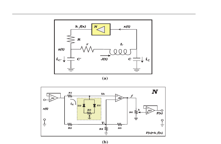
Fig. 6. (a) The circuit diagram of a nonlinear chaotic oscillator. The component values
employed are C
�
= 100.2 nF, C = 200.1 nF, L = 63.8 mH, r = 138.9 Ω, and R = 1018 Ω. (b)
Schematic diagram of the nonlinear converter N. The electronic component values are
R1
= 2.7 kΩ, R2 = R4 = 7.5 kΩ, R3 = 50 Ω, R5 = 177 kΩ, R6 = 20 k Ω. The diodes D1 and
D2 are 1N4148, the operational amplifiers A1 and A2 are both TL082, and the operational
amplifier A3 is LF356N.
a shape similar to a Rössler oscillator (Fig. 7(a)), and to a double scroll oscillator (Fig. 7(b)).
They can be easily obtained by just fixing the bifurcation paramete r k to be equal to 0.4010,
and 0.3964, re spectively.
4.2 Wavelet variance
In the wavelet approach the fractal character of a certain signal can be inferred from the
behavior of its power spectrum P
(ω), which is the F ourier transform of the autocorrelation
function and i n differential form P
(ω)dω represents the contribution to the variance of the
part of the signal contained between frequencies ω and ω
+ dω. Indeed, it is known that for
self-similar random processes the spectral behavior of the power spectrum is given by
P
(ω) ∼| ω |
−β
, (21)
where β is the spectral parameter of the signal. In addition, the variance of the wavelet
coefficients var
{d
m
n
} is related to the level m through a p ower law of the type (Wor nell &
Oppenheim, 1992)
14
Discrete Wavelet Transforms - Theory and Applications
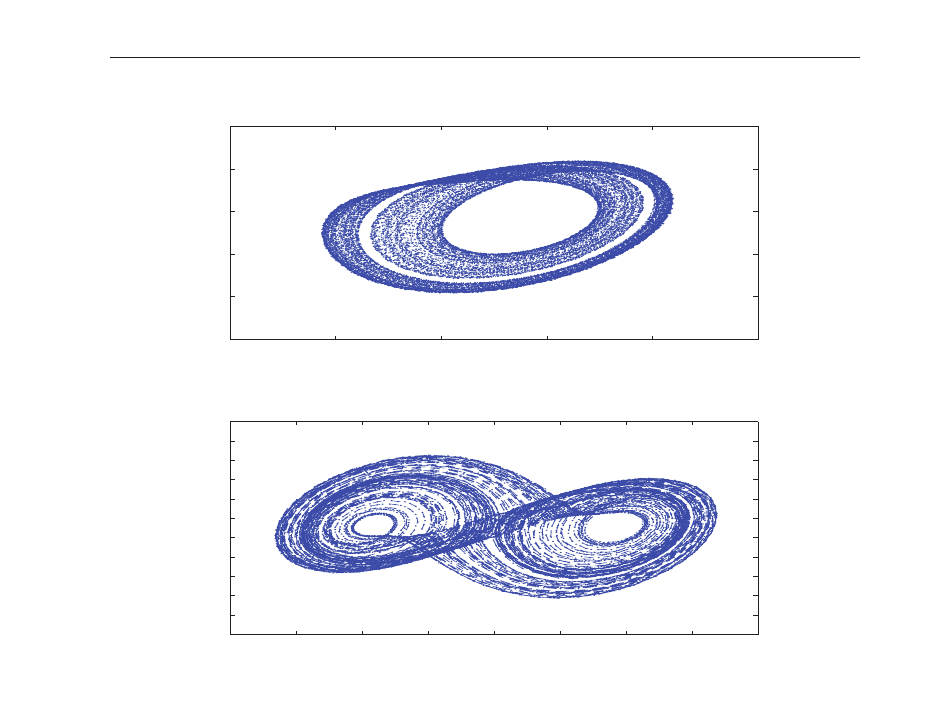
Fig. 6. (a) The circuit diagram of a nonlinear chaotic oscillator. The component values
employed are C
�
= 100.2 nF, C = 200.1 nF, L = 63.8 mH, r = 138.9 Ω, and R = 1018 Ω. (b)
Schematic diagram of the nonlinear converter N. The electronic component values are
R1
= 2.7 kΩ, R2 = R4 = 7.5 kΩ, R3 = 50 Ω, R5 = 177 kΩ, R6 = 20 k Ω. The diodes D1 and
D2 are 1N4148, the operational amplifiers A1 and A2 are both TL082, and the operational
amplifier A3 is LF356N.
a shape similar to a Rössler oscillator (Fig. 7(a)), and to a double scroll oscillator (Fig. 7(b)).
They can be easily obtained by just fixing the bifurcation paramete r k to be equal to 0.4010,
and 0.3964, re spectively.
4.2 Wavelet variance
In the wavelet approach the fractal character of a certain signal can be inferred from the
behavior of its power spectrum P
(ω), which is the F ourier transform of the autocorrelation
function and i n differential form P
(ω)dω represents the contribution to the variance of the
part of the signal contained between frequencies ω and ω
+ dω. Indeed, it is known that for
self-similar random processes the spectral behavior of the power spectrum is given by
P
(ω) ∼| ω |
−β
, (21)
where β is the spectral parameter of the signal. In addition, the variance of the wavelet
coefficients var
{d
m
n
} is related to the level m through a p ower law of the type (Wor nell &
Oppenheim, 1992)
−2 −1.5 −1 −0.5 0 0.5 1 1.5 2
−1
−0.8
−0.6
−0.4
−0.2
0
0.2
0.4
0.6
0.8
1
x
(b)
−0.5 0 0.5 1 1.5 2
−1.5
−1
−0.5
0
0.5
1
y
(a)
Fig. 7. Attractors o f the electronic chaotic circuit projected on the plane x −y obtained
experimentally for two different values of the bifurcation parameter k: (a) 0.4010, and (b)
0.3964.
var
{d
m
n
}≈(2
m
)
−β
. (22)
This wavelet variance has been used to find dominant levels associated with the signal, for
example, i n the stud y of numerical and experime ntal chaotic time series ( Campos-Cantón et
al., 2008; Murguía & Campos-Cantón, 2006; Staszewski & Worden, 1999). In order to estimate
β we used a least squares fit of the linear model
log
2
(var{d
m
n
} )=β
m
+(K + v
m
), (23)
where K and v
m
are constants relate d to the linear fitting procedure. Equation (22) is
certainly suitable for studying discrete chaotic time serie s, because their variance plot has a
well-defined form as pointed out in (Murguía & Campos -Cantón, 2006; Staszewski & Worden,
1999). If the variance plot shows a maximum at a particular scale, or a bump over a group
of scales, which means a high energy concentration, it will often correspond to a coherent
15
Discrete Wavelet Analyses for Time Series

structure. In general, the gradient of a noisy time series turns out to be zero in the variance
plot, therefore it does not show any energy concentration at specific wavelet level. In certain
cases the gradient of so me chaotic time series has a similar appearance with Gaussi an noise
at lower scales, which implies that these chaotic time series do not present a fundamental
“carrier” frequency at any scale.
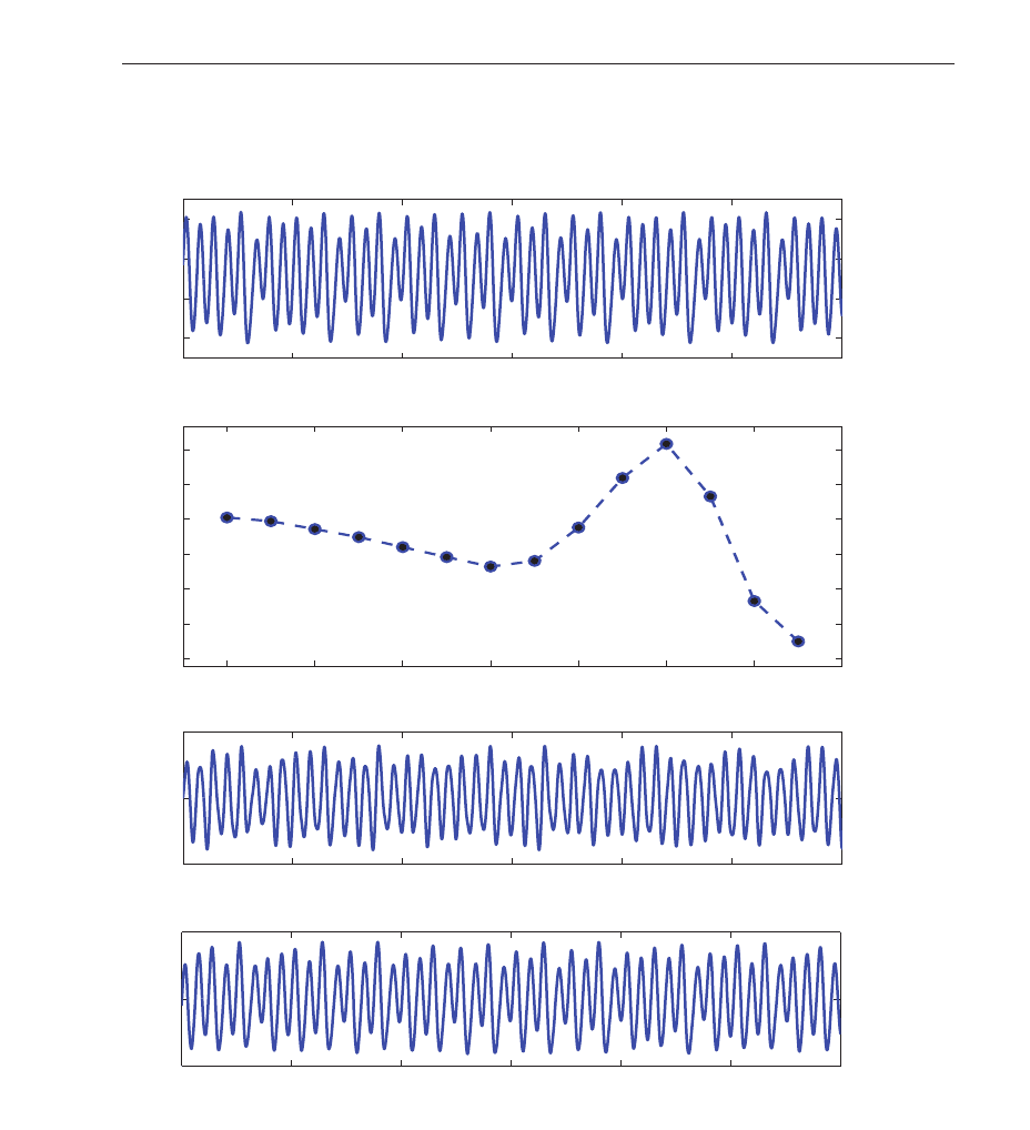
For our illustrative analysis and comparison with the experiments, we study the time series
of the x states of the attractors displayed in Fig. 7(a)-(b), because they are of ver y different
type and we want to emphasize the versatility of the wavelet approach. The acquisition of
the exper imental data was carr ied out with a DAQ with a sam pling f requency of 180 kHz, i.e.
we collected the experimental data for a total time of 182 ms for both si gnals. In the analysis
of these time series we employ ed the db-8 wavelet, a wavelet function that belo ngs to the
Daubechies family (Daubechies, 1992; Mallat, 1999).
• Case k
= 0.4010.
The first time series to consider corresponds to the x state o f the experimental attractor
of Fig. 7 (a). The first 12 ms of this time series are shown in Fig. 8 (a), whereas Fig. 8 (b)
shows a semi-logarithmic plot of the wavelet coefficient variance as a function of level m,
which is denominated as variance plot of the wavelet coefficients. One can notice that the
whole series is dominated by the 12th wavelet level, i.e., this wavelet level has the major
energy concentration, and it is plotted in isolation in Fig. 8 (c). The energy rate between the
reconstructed signal with respect to the original signal w as
(E
x
12
/E
x
)=0.9565, which
means an energy close to 96% of the total one in this case. Since it does not properly
show the structure of the chaotic time serie s, we considered and added together the three
neighbor wavelet levels, m
= 11 − 13, achieving an energy concentration of 99% of the
total one. In this case, the reconstructio n of the signal at these wavelet levels is shown in
Fig. 8(d), where the structure o f the original sig nal can be noticed. Both reconstructed time
series present a slight downward translation, because of the DC component of this chaotic
time series.
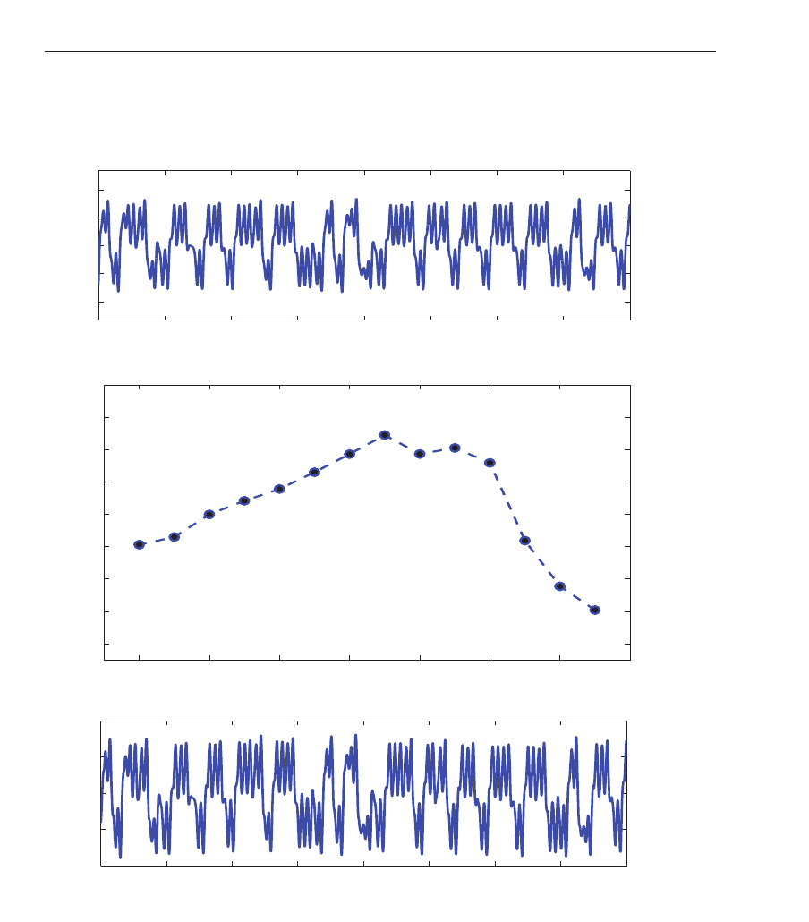
• Case k
= 0.3964.
For this value of k, the behaviour of the chaotic electronic circuit is similar to that of a
double scroll oscillator with the shape of the attractor displayed in Fig. 7. The experimental
time series corresponding to the x state of this attractor is shown in Fig. 9 (a), while the
variance plot is given in Fig. 9 (b) where the gradient is close to zero , which means that
no significant energy concentration can be seen. We have found that when summing over
the wavelet levels m
= 6 − 12 the energy concentration is close to 99% of the total one but
without any prono unced peak. T hus, this case does not present a fundamental “carrier”
frequency and therefore this attractor has a Gaussian noisy behavio r. The reconstructed
time series with the mentioned wavelet levels is displayed in Fig. 9 (c).
5. Conclusion
The DWT is currently a standard tool to study time-series produced by all sorts of
non-stationary dynamical system s. In this chapter, we first revie w ed the main properties of
DWT and the basic concepts re lated to the corresponding mathematical formalism. Next, we
presented the way the DWT characterizes the type of dynamics embedded in the time-series.
In general, the DWT reveals with high accuracy the dynamical features obeying power-l ike
scaling properties of the processed s ignals and has been already successfully incorporated in
the multifractal formalism. The interesting case of the time-series of the elementary cellular
0 2 4 6 8 10 12
0
0.5
1
1.5
t(ms)
x(V)
(a)
2 4 6 8 10 12 14 16
−14
−12
−10
−8
−6
−4
−2
m
log | var ( d
n
m
) |
(b)
0 2 4 6 8 10 12
−1
0
1
t(ms)
x
m=12
(V)
(c)
0 2 4 6 8 10 12
−1
0
1
t(ms)
x
m=11�13
(V)
(d)
Fig. 8. The case k = 0.4010: (a) exper imental time series of the x state, (b) wavelet coefficient
variance, (c) time series of the 12th wavelet level, and (d) the time series of the sum from 11th
to the 13th wavelet levels.
16
Discrete Wavelet Transforms - Theory and Applications
structure. In general, the gradient of a noisy time series turns out to be zero in the variance
plot, therefore it does not show any energy concentration at specific wavelet level. In certain
cases the gradient of some chaotic time series has a similar appearance with Gaussi an noise
at lower scales, which implies that these chaotic time series do not present a fundamental
“carrier” frequency at any scale.
For our illustrative analysis and comparison with the experiments, we study the time series
of the x states of the attractors displayed in Fig. 7(a)-(b), because they are of ver y different
type and we want to emphasize the versatility of the wavelet approach. The acquisition of
the exper imental data was carr ied out with a DAQ with a sam pling f requency of 180 kHz, i.e.
we collected the experimental data for a total time of 182 ms for both si gnals. In the analysis
of these time series we employ ed the db-8 wavelet, a wavelet function that belo ngs to the
Daubechies family (Daubechies, 1992; Mallat, 1999).
• Case k
= 0.4010.
The first time series to consider corresponds to the x state o f the experimental attractor
of Fig. 7 (a). The first 12 ms of this time series are shown in Fig. 8 (a), whereas Fig. 8 (b)
shows a semi-logarithmic plot of the wavelet coefficient variance as a function of level m,
which is denominated as variance plot of the wavelet coefficients. One can notice that the
whole series is dominated by the 12th wavelet level, i.e., this wavelet level has the major
energy concentration, and it is plotted in isolation in Fig. 8 (c). The energy rate between the
reconstructed signal with respect to the original signal w as
(E
x
12
/E
x
)=0.9565, which
means an energy close to 96% of the total one in this case. Since it does not properly
show the structure of the chaotic time serie s, we considered and added together the three
neighbor wavelet levels, m
= 11 − 13, achieving an energy concentration of 99% of the
total one. In this case, the reconstructio n of the signal at these wavelet levels is shown in
Fig. 8(d), where the structure o f the original sig nal can be noticed. Both reconstructed time
series present a slight downward translation, because of the DC component of this chaotic
time series.
• Case k
= 0.3964.
For this value of k, the behaviour of the chaotic electronic circuit is similar to that of a
double scroll oscillator with the shape of the attractor displayed in Fig. 7. The experimental
time series corresponding to the x state of this attractor is shown in Fig. 9 (a), while the
variance plot is given in Fig. 9 (b) where the gradient is cl ose to zero, which means that
no significant energy concentration can be seen. We have found that when summing over
the wavelet levels m
= 6 − 12 the energy concentration is close to 99% of the total one but
without any prono unced peak. T hus, this case does not present a fundamental “carri er”
frequency and therefore this attractor has a Gaussian noisy behavio r. The reconstructed
time series with the mentioned wavelet levels is displayed in Fig. 9 (c).
5. Conclusion
The DWT is currently a standard tool to study time-series produced by all sorts of
non-stationary dynamical system s. In this chapter, we first revie w ed the main properties of
DWT and the basic concepts re lated to the corresponding mathematical formalism. Next, we
presented the way the DWT characterizes the type of dynamics embedded in the time-series.
In general, the DWT reveals with high accuracy the dynamical features obeying power-l ike
scaling properties of the processed s ignals and has been already successfully incorporated in
the multifractal formalism. The interesting case of the time-series of the elementary cellular
0 2 4 6 8 10 12
0
0.5
1
1.5
t(ms)
x(V)
(a)
2 4 6 8 10 12 14 16
−14
−12
−10
−8
−6
−4
−2
m
log | var ( d
n
m
) |
(b)
0 2 4 6 8 10 12
−1
0
1
t(ms)
x
m=12
(V)
(c)
0 2 4 6 8 10 12
−1
0
1
t(ms)
x
m=11�13
(V)
(d)
Fig. 8. The case k = 0.4010: (a) exper imental time series of the x state, (b) wavelet coefficient
variance, (c) time series of the 12th wavelet level, and (d) the time series of the sum from 11th
to the 13th wavelet levels.
0 2 4 6 8 10 12
0
0.5
1
1.5
t(ms)
x(V)
(a)
2 4 6 8 10 12 14 16
−14
−12
−10
−8
−6
−4
−2
m
log | var ( d
n
m
) |
(b)
0 2 4 6 8 10 12
−1
0
1
t(ms)
x
m=12
(V)
(c)
0 2 4 6 8 10 12
−1
0
1
t(ms)
x
m=11�13
(V)
(d)
Fig. 8. The case k = 0.4010: (a) exper imental time series of the x state, (b) wavelet coefficient
variance, (c) time series of the 12th wavelet level, and (d) the time series of the sum from 11th
to the 13th wavelet levels.
17
Discrete Wavelet Analyses for Time Series
0 5 10 15 20 25 30 35 40
−2
−1
0
1
2
t(ms)
x(V)
(a)
2 4 6 8 10 12 14 16
−14
−12
−10
−8
−6
−4
−2
0
2
m
log | var ( d
n
m
) |
(b)
0 5 10 15 20 25 30 35 40
−2
−1
0
1
2
t(ms)
x
m = 6�12
(V)
(c)
Fig. 9. The case k = 0.3964: (a) exper imental time series of the x state, (b) wavelet coefficient
variance, (c) time series of the sum from 6th to the 12th wavelet l evels.
0 5 10 15 20 25 30 35 40
−2
−1
0
1
2
t(ms)
x(V)
(a)
2 4 6 8 10 12 14 16
−14
−12
−10
−8
−6
−4
−2
0
2
m
log | var ( d
n
m
) |
(b)
0 5 10 15 20 25 30 35 40
−2
−1
0
1
2
t(ms)
x
m = 6�12
(V)
(c)
Fig. 9. The case k = 0.3964: (a) exper imental time series of the x state, (b) wavelet coefficient
variance, (c) time series of the sum from 6th to the 12th wavelet l evels.
18
Discrete Wavelet Transforms - Theory and Applications