Nof S.Y. Springer Handbook of Automation
Подождите немного. Документ загружается.


Economic Aspects of Automation 6.4 Mid-Term Effects of Automation 105
proportion – as stated by markup theory – only in the
particular case of (6.35b). In the other cases the transla-
tion results less than proportional, as the sought markup
decreases as w increases.
Nominal Prices and Wages: Some Conclusions
Elasticity of product price decreases if the term
ˆ
vP
0
K
ˆ
λ/w increases, representing the ratio between the
nominal value of capital (P
0
K
¯
K) and labor cost (wL).
Since automation necessarily implies a remarkable in-
crease of this ratio, it results in minor prices sensibility
to wages variation. In practice, automation implies
beneficial effects on inflation: for increasing nominal
wages, a high-capital-intensity economy is less subject
to inflation shocks caused by wage rises.
6.4.2 Macroeconomics Effects
of Automation in the Mid-Term:
Actual Wages
and Natural Unemployment
In order to analyze effects of automation on macroeco-
nomic balance in the mid term, it is necessary to convey
the former equations of prices in terms of real wages,
dividing each member by P, in order to take account
of ω = w/P, which represents the maximum wage that
firms are prepared to pay to employees without giving
up their desired profit rate.
1. Keeping physical capital intact (P
0
K
= P
K
= p
k
P)
ω
a
=
ˆ
λ[1−(d+r
∗
)
ˆ
v p
k
]=
ˆ
λ/
1+μ
∗
a
(6.37a)
2. Wholeness of capital granted by owners (P
K
=
p
k
P> P
0
K
)
ω
b
=
ˆ
λ
1−(d+r
∗
)
ˆ
v
p
k
−l
∗
p
k
−P
0
K
/P
(6.37b)
3. Recovery of capital’s nominal value (P
K
= P
0
K
)
ω
c
=
ˆ
λ
1−(d+r
∗
)
ˆ
vP
0
K
/P
(6.37c)
In the borderline case of keeping physical capital
intact (6.37a) only one level of real salary ω
a
exists
consistent with a specified level of capital productiv-
ity r
∗
, given work productivity
ˆ
λ, amortization rate d,
capital/product ratio
ˆ
v (corresponding to normal use of
plants), and relative price p
k
of capital with respect to
product.
The value of ω
a
can also be expressed as a link
between work productivity and profit margin factor
(1+μ
∗
a
) with variable costs, assuming that the desired
markup is unchanging in comparison with prices.
In the rational case of corporate stock integrity and
in the generally adopted case of recovery of capital
nominal value, an increasing relation exists between
real salary and general price level, with the desired
markup being variable, as shown in connections (6.36b)
and (6.36c).
The elasticity of ω with respect to P turns out to
increase from (6.37a)to(6.37c)
η
a
=(∂ω/∂P)(P/ω) =0
<η
b
=(
ˆ
λ/ω
b
)l
∗
(d+r
∗
)
ˆ
vP
0
K
/P
<η
c
=(
ˆ
λ/ω
c
)(d +r
∗
)
ˆ
vP
0
K
/P
=
ˆ
λ/ω
c
−1
<
>
1 with ω
c
>
<
ˆ
λ/2 .
(6.37d)
In cases 2 and 3 growth in the prices general level
raises the added value share intended for normal cap-
ital remuneration, leaving firms a markup to be used
in bargaining in order to grant employees a pay rise in
real salary, even while keeping normal profit rate (the
calculated level with programmed production) steady.
This markup of real wage bargaining depends on
the choice of the capital recovery system: it is higher in
the case of fund illusion and lower in the case in which
capital stock is intended to be maintained undivided.
Remark: In all three cases above, the level of real
salary depends on the degree of production process
automation: in economic systems where this is high,
productivity of work (
ˆ
λ) and capital (1/
ˆ
v) are neces-
sarily higher than the related price of capital (p
k
and
P
0
K
/P), so the real wage that the firms are willing
to concede in bargaining is higher than the one af-
fecting work-intensive economic systems. In substance,
automation weakens firms’ resistance in wage bargain-
ing, making them more willing to concede higher real
wages.
In order to qualify the positive role of automa-
tion we complete the mid-term period macroeconomic
model with the wage equation from the workers’ side.
Macroeconomics theory believes that, in the mid
term, nominal wages w asked for by workers in syn-
dicated or individual bargaining (or imposed by firms in
order to select and extract optimal effort in production
process) depend on three variables: the unemployment
rate of man power u, other factors absorbed in a syn-
thetic variable z, and the expected level of prices P
e
.
So it is possible to write
w =ω(u, z)P
e
. (6.38)
Part A 6.4
106 Part A Development and Impacts of Automation
Higher unemployment is supposed to weaken workers’
contractual strength, compelling them to accept lower
wages, and vice versa that a decrease of unemploy-
ment rate leads to requests for an increase of real wages
(∂ω/∂u < 0).
The variable z can express the effects of unemploy-
ment increase, which would compel workers to ask for
a pay raise, because any termination would appear less
riskyintermsofsocial salary (the threshold above
which an individual is compelled to work and under
which he is not prepared to accept, at worst choos-
ing unemployment). Similar effects would be induced
by legal imposition of minimum pay and other forms
of worker protection, which – making discharge more
difficult – would strengthen workers’ position in wage
bargaining.
Regarding the expected level of prices, it is sup-
posed that
∂w/∂P
e
=w/P
e
> 0 ⇒(∂w/∂P
e
)(P
e
/w) =1
to point out that rational subjects are interested in
real wages (their buying power) and not nominal ones,
so an increase in general level of prices would bring
about an increase in nominal wages in the same pro-
portion. Wages are however negotiated by firms on
nominal terms, on the basis of a price foresight (P
e
)for
the whole length of the contract (generally more than
1year), during which monetary wages are not corrected
if P = P
e
.
To accomplish this analysis, in the mid-term period,
wage bargaining is supposed to have real wage as a sub-
ject (excluding systematic errors in expected inflation
foresight), so that P = P
e
and (6.38) can be simplified
to
ω =ω(u, z) .
(6.39)
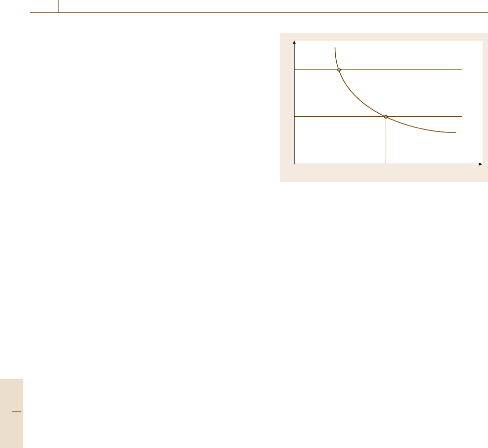
Figure 6.2 illustrates this relation with a decreasing
curve WS (wage setting), on Cartesian coordinates for
agivenlevelofz.
Two straight lines, PS (price setting), representing
price equations (6.37a), considering mainly the bor-
derline case of maintaining physical capital intact, are
reported:
•
The upper line PS
A
refers to an economic sys-
tem affected by a high degree of automation, or
by technologies where θ
k
=1 and work and capi-
tal productivity are higher, being able to contrast the
capital’s relative higher price; in this case firms are
prone to grant higher real wages.
u
A
n
u
a
n
E
a
E
A
PS
A
PS
a
WS(z)
u
ω
0
Fig. 6.2 Mid-term equilibrium with high and low automa-
tion level
•
The lower line PS
a
, characterizing an economy with
a lower degree of automation, resulting in less will-
ingness to grant high real wages.
The intersection between the curve WS and the line PS
indicates one equilibrium point E for each economic
system (where workers’ plans are consistent with those
of firms), corresponding to the case in which only one
natural unemployment rate exists, obtained by balanc-
ing (6.37a)and(6.39)
ˆ
λ
1−(d+r
∗
)
ˆ
v p
k
=ω(u, z) ⇒u
A
n
< u
a
n
, (6.40a)
assuming that [1−(d +r
∗
)
ˆ
v p
k
]d
ˆ
λ −
ˆ
λ(d +r
∗
)p
k
d
ˆ
v>
ˆ
λ(d +r
∗
)
ˆ
vdp
k
.
Remark: In the case of a highly automated system,
wage bargaining in the mid-term period enables a natu-
ral unemployment rate smaller than that affecting a less
automated economy: higher productivity makes enter-
prises more willing to granthigher real wages as a result
of bargaining and the search for efficiency in produc-
tion organizations, so that the economic system can
converge towards a lower equilibrium rate of unemploy-
ment (u
A
n
< u
a
n
).
The uniqueness of this solution is valid only if en-
terprises aim to maintain physical capital undivided.
In the case of rational behavior intended to achieve
the integrity of capital stock alone (6.37b), or business
procedures oriented to recoup the accounting value of
capital alone (6.37c), the natural unemployment rate
theory is not sustainable. In fact, if we equalize these
two relations to (6.39), respectively, we obtain in both
cases a relation describing balance couples between un-
employment rate and prices general level, indicating
that the equilibrium rate is undetermined and therefore
Part A 6.4
Economic Aspects of Automation 6.4 Mid-Term Effects of Automation 107
that the adjective natural is inappropriate
ˆ
λ
1−(d+r
∗
)
ˆ
v
p
k
−l
∗
p
k
−P
0
K
/P
=ω(u, z)
⇒u
n
=u
b
n
(P) , (6.40b)
ˆ
λ
1−(d+r
∗
)
ˆ
vP
0
K
/P
=ω(u, z)
⇒u
n
=u
c
n
(P) , (6.40c)
where ∂u
n
/∂P < 0, since an increase in P increases
the margin necessary to recover capital cost and so
enterprises can pay out workers a higher real salary
(∂ω/∂P> 0), which in balance is compatible with
a lower rate of unemployment.
Summing up, alternative enterprise behavior to that
intended to maintain physical capital intact does not
allow fixing univocally the natural rate of unemploy-
ment. In fact,highly automated economicsystems cause
a translation of the function u
n
= u
n
(P)toalower
level: for an identical general level of prices the unem-
ployment balance rate is lower since automation allows
increased productivity and real wage that enterprises are
prepared to pay.
6.4.3 Macroeconomic Effects
of Automation in the Mid Term:
Natural Unemployment
and Technological Unemployment
The above optimistic conclusion of mid-term equi-
librium being more profitable for highly automation
economies must be validated in the light of constraints
imposed by capital-intensive technologies, where the
production rate is higher and yields are constant.
Assume that in the economic system an aggregated
demand is guaranteed, such that all production volumes
could be sold, either owing to fiscal and monetary poli-
tics oriented towards full employment or hoping that, in
the mid term, the economy will spontaneously converge
through monetary adjustments induced by variation of
the price general level.
In a diffused automation context, a problem could
result from a potential inconsistency between the unem-
ployment natural rate u
n
(obtained byimposing equality
of expected and actual prices, related to labor market
equilibrium) and the unemployment rate imposed by
technology
¯
u
¯
u = 1−L
d
/L
s
=1−(
¯
Y/
ˆ
λ)/L
s
>
<
u
n
, (6.41)
where L
d
=
¯
Y/
ˆ
λ is the demand for labor, L
s
is the labor
supply, and
¯
Y is the potential production rate, compati-
ble with full utilization of production capacity.
A justification of this conclusion can be seen by
noting that automation calls for qualified technical per-
sonnel, who are still engaged by enterprises even during
crisis periods, and of whom overtime work is required
in case of expansion. Then, employment variation is
not proportional to production variation, as clearly re-
sults from the law of Okun [6.45], and from papers by
Perry [6.46]andTatom [6.47].
Remark: From the definition of
¯
u it follows that
economic systems with high automation level, and
therefore characterized by high productivity of labor,
present higher technological unemployment rates
(∂
¯
u/∂
ˆ
λ)(
ˆ
λ/
¯
u) =(1−
¯
u)/
¯
u > 0 .
On one hand, automation reduces the natural unemploy-
ment rate u
n
, but on the other it forces the technological
unemployment rate
¯
u to increase. If it holds that
¯
u ≤u
n
,
the market isdominant and theeconomic systemaims to
converge in time towards an equilibrium characterized
by higher real salary and lower (natural) unemploy-
ment rate,as soonas thebeneficial effects of automation
spread.
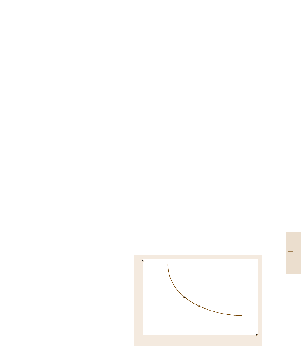
In Fig.6.3, the previous Fig.6.2 is modified un-
der the hypothesis of a capital-intensive economy, by
including twovertical lines corresponding to two poten-
tial unemployment rates imposed by technology (
¯
u and
¯
u
A
). Note that
¯
u has been placed on the left of u
n
whilst
¯
u
A
has been placed on the right of u
n
. It can be seen
that the labor market equilibrium (point E) dominates
when technology implies a degree of automation com-
patible with a nonconstraining unemployment rate
¯
u.
Equilibrium could be obtained, on the contrary, when
technology (for a given production capacity of the eco-
u
A
uu
n
E
H
PS
A
WS(z)
u
ω
0
Fig. 6.3 Mid-term equilibrium with high automation level
and two different technological unemployment rates
Part A 6.4

108 Part A Development and Impacts of Automation
nomic system) cannot assure a low unemployment rate:
¯
u
A
> u
n
.
The technological unemployment constraint implies
a large weakness when wages are negotiated by work-
ers, and it induces a constrained equilibrium (point H)
in which the real salary perceived by workers is lower
than that which enterprises are willing to pay. The latter
can therefore achieveunplanned extra profits,so thatau-
tomation benefits only generate capital owners’ income
which, in the share market, gives rise to share value
increase.
Only a relevant production increase and equivalent
aggregated demand could guarantee a reduction of
¯
u
A
,
thus transferring automation benefits also to workers.
These conclusions can have a significant im-
pact on the Fisher–Phillips curve (Fisher [6.48]
and Phillips [6.49], first; theoretically supported by
Lipsey [6.50] and then extended by Samuelson and
Solow [6.51]) describing the trade-off between inflation
and unemployment.
Assume that the quality constraint between ex-
pected prices and effective prices can, in the mid term,
be neglected, in order to analyze the inflation dynamics.
Then, substitute (6.38)into(6.35b), by assuming thehy-
pothesis that maintaining capital intact implies constant
markup
P = (1+μ
∗
)ω(u, z)P
e
/
ˆ
λ. (6.42)
This relation shows that labor market equilibrium for
imperfect information (P
e
= P), implies a positive link
between real and expected prices.
By dividing (6.42)byP
−1
, the following relation
results
1+π = (1+π
e
)(1+μ
∗
)ω(u, z)/
ˆ
λ, (6.43a)
where:
•
π = P/P
−1
−1 is the current inflation rate
•
π
e
= P
e
/P
−1
−1 is the expected inflation rate.
Assume moderate inflation rates, such that
(1+π)/(1+π
e
) ≈1+π −π
e
and consider a linear relation between productivity and
wages, such that it amounts to 100% if
z = u = 0 :ω(u, z)/
ˆ
λ =1+α
0
z−α
1
u(α
0
,α
1
> 0) .
Relation (6.43a) can be simplified to
π =π
e
+(1+μ
∗
)α
0
z−(1+μ
∗
)α
1
u , (6.43b)
which is a linearversion ofthe Phillips curve; according
to this form, the current inflationrate depends positively
on inflation expectation, markup level, and the variable
z, and negatively on the unemployment rate.
For π
e
=0, the original curve which Phillips and
Samuelson–Solow estimated for the UK and USA is
obtained.
For π
e
= π
−1
(i.e., extrapolative expectations)
a link between the variation of inflation rate and the
unemployment rate (accelerated Phillips curve), show-
ing better interpolation of data observed since 1980s, is
derived
π −π
−1
=(1+μ
∗
)α
0
z−(1+μ
∗
)α
1
u . (6.44)
Assuming π = π
e
= π
−1
in (6.43b)and(6.44), an
estimate of the natural unemployment rate (without sys-
tematic errors in mid-term forecasting) can be derived
u
n
=α
0
z/α
1
. (6.45)
Now, multiplying and dividing by the α
1
term (1+
μ
∗
)α
0
z in (6.44), and inserting (6.45)into(6.44), it re-
sults that, in the case of extrapolative expectations,the
inflation rate reduces if the effective unemployment rate
is greater than the natural one (dπ<0ifu > u
n
); it in-
creases in the opposite case (dπ>0ifu < u
n
); and it
is zero (constant inflation rate) if the effective unem-
ployment rate is equal to the natural one (dπ = 0if
u = u
n
)
π −π
−1
=−(1+μ
∗
)α
1
(u −u
n
) . (6.46)
Remark: Relation (6.44) does not take into account
effects induced by automation diffusion, which imposes
on the economic system a technological unemployment
¯
u
A
that increases with increasing automation.
It follows that any econometric estimation based
on (6.44) no longer evaluates the natural unemployment
rate (6.45)forπ −π
−1
=0, because the latter varies in
time, flattening the interpolating line (increasingly high
unemployment rates related to increasingly lower real
wages, as shown above). Then, as automation process
spreads, the natural unemployment rate (which, with-
out systematic errors, assures compatibility between the
real salary paid by enterprises and the real salary ei-
ther demanded by workers or supplied by enterprises
for efficiency motivation) is no longer significant.
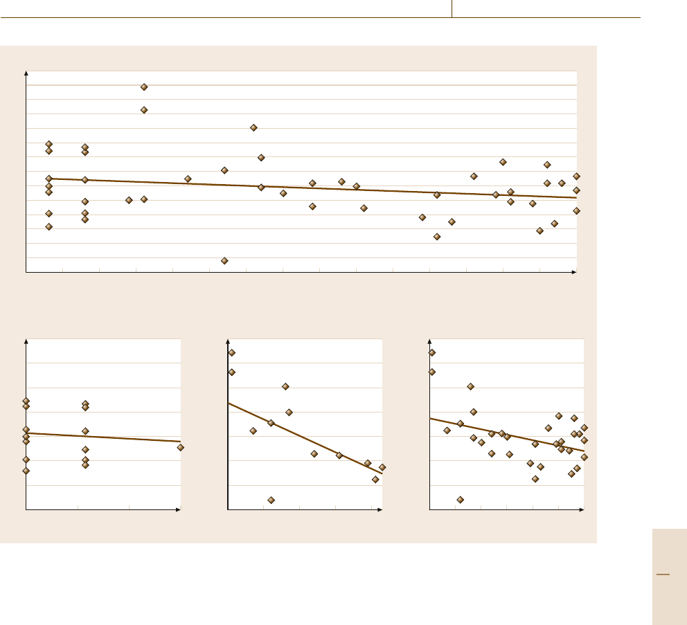
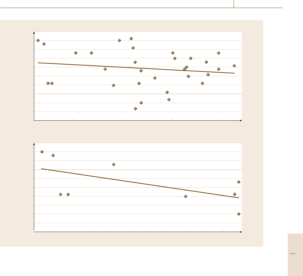
In Fig.6.4a the Phillips curve for the Italian eco-
nomic system, modified by considering inflation rate
variations from 1953 to 2005 and the unemployment
rate, is reported; the interpolation line is decreasing but
very flat owing to
¯
u
A
movement towards the right.
A natural unemployment rate between 7 and 8%
seems to appear, but the intersection of the interpola-
tion line with the abscissa is moved, as shown in the
Part A 6.4
Economic Aspects of Automation 6.4 Mid-Term Effects of Automation 109
4.5 5 5.5 6 6.5 7 7.5 8 8.5 9 9.5 10 10.5 11 11.5 12
Inflation rate variation (%)
Unemployment rate (%)
8
7
6
5
4
3
2
1
0
–1
–2
–3
–4
–5
–6
4.8 5.2 5.6 6
Inflation rate variation (%)
a) Economic miracle: 1953–1972
Unemployment rate (%)
8
6
4
2
0
–2
–4
–6
678910
Inflation rate variation (%)
b) Petroleum shock: 1973–1985
Unemployment rate (%)
8
6
4
2
0
–2
–4
–6
6789101112
Inflation rate variation (%)
c) 1973–2005
Unemployment rate (%)
8
6
4
2
0
–2
–4
–6
Fig. 6.4a–c Italy: Expectations-augmented Phillips curve (1953–2005). (a) Economic miracle: 1953–1972,
(b) petroleum shock: 1973–1985, (c) 1973–2005
three representations where homogeneous data sets of
the Italian economic evolution are considered.
Automation has a first significant impact during the
oil crisis, moving the intersection from 5.2% for the
first post-war 20 years up to 8% in the next period. Ex-
tending the time period up to 2005, intersection moves
to 9%; the value could be greater, but it has been re-
cently bounded by the introduction of temporary work
contracts which opened new labor opportunities but
lowered salaries.
Note that Figs. 6.4a–c are partial reproductions of
the Fig. 6.4, considering three different intervals of un-
employment rate values. This reorganization of data
corresponds to the three different periods of the Italian
economic growth: (a) the economic miracle (1953–
1972), (b)the petroleumshock (1973–1985),and (c) the
period from the economic miracle until 2005 (1973–
2005).
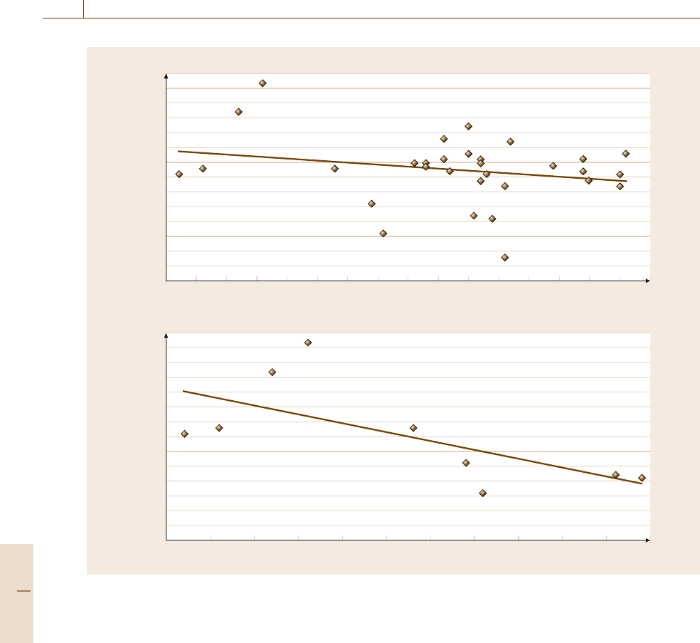
A more limited but comprehensive analysis, ow-
ing to lack of homogeneous historical data over the
whole period, has been done also for two other impor-
tant European countries, namely France (Fig.6.5a) and
Germany (Fig.6.5b): the period considered ranges from
1977 to 2007.
The unemployment rate values have been recom-
puted so as to make all the historical series homoge-
neous. Owing to the limited availability of data for both
countries, only two periods have been analyzed: the
period 1977–1985, with the effects of the petroleum
shock, and the whole period up to 2007, in order to
Part A 6.4
110 Part A Development and Impacts of Automation
4 4.5 5 5.5 6 6.5 7 7.5 8 8.5 9 9.5 10 10.5 11 11.5 12
a) Inflation rate variation (%) France: Expectations-augmented Phillips curve (1977–2007)
Unemployment rate (%)
3
2.5
2
1.5
1
0.5
0
–0.5
–1
–1.5
–2
–2.5
–3
–3.5
–4
4 4.5 5 5.5 6 6.5 7 7.5 8 8.5 9 9.5
Inflation rate variation (%) France: Petroleum shock: 1977–1985
Unemployment rate (%)
3
2.5
2
1.5
1
0.5
0
–0.5
–1
–1.5
–2
–2.5
–3
–3.5
–4
Fig. 6.5 (a) France: expectations-augmented Phillips curve (1977–2007) (b) Germany: expectations-augmented
Phillips curve (1977–2007)
evaluate the increase of the natural unemployment rate
from the intersection of the interpolation line with the
abscissa.
As far as Fig.6.5a is concerned, the natural unem-
ployment rate is also increased in France – as in Italy –
by more than one percentage point (from less than 6%
to more than 7%). In the authors’ opinion, this increase
should be due to technology automation diffusion and
consequent innovation of organization structures.
Referring to Fig.6.5b, it can be noted that even in
Germany the natural unemployment rate increased –
more than in France and in Italy – by about three per-
centage points (from 2.5to5.5%). This effect is partly
due to application of automated technologies (which
should explain about one percentage point, as in the
other considered countries), and partly to the reunifica-
tion of the two parts of German.
A Final Remark: Based on the considerations and
data analysis above it follows that the natural unem-
ployment rate, in an industrial system where capital
intensive enterprises are largely diffused, is no longer
significant, because enterprises do not apply methods
to maintain capital intact, and because technological
inflation tends to constraint the natural one.
Only structural opposing factors could slow this
process, such as labor market reform, to give rise to
new work opportunities, and mainly economic poli-
tics, which could increase the economy development
Part A 6.4
Economic Aspects of Automation 6.5 Final Comments 111
0.5 1 1.5 2 2.5 3 3.5 4 4.5 5 5.5 6 6.5 7 7.5 8 8.5 9 9.5 10 10.5 11
b) Inflation rate variation (%) Germany: Expectations-augmented Phillips curve (1977–2007)
Unemployment rate (%)
2
1.5
1
0.5
0
–0.5
–1
–1.5
–2
–2.5
–3
2
1.5
1
0.5
0
–0.5
–1
–1.5
–2
–2.5
–3
0.5 1 1.5 2 2.5 3 3.5 4 4.5 5 5.5 6
Inflation rate variation (%) Germany: Petroleum shock: 1977–1985
Unemployment rate (%)
trend more than the growth of productivity and labor
supply. However, these aspects should be approached
in a long-term analysis, and exceed the scope of this
chapter.
6.5 Final Comments
Industrial automation is characterized by dominance
of capital dynamics over the biological dynamics of
human labor, thus increasingthe production rate. There-
fore automation plays a positive role in reducing costs
related to both labor control, sometimes making mon-
etary incentives useless, and supervisors employed to
assure the highest possible utilization of personnel. It is
automation itself that imposes the production rate and
forces workers to correspond to this rate.
In spite of these positive effects on costs, the in-
creased capital intensity implies greater rigidity of
the cost structure: a higher capital cost depending on
higher investment value, with consequent transforma-
tion of some variable costs into fixed costs. This induces
a greater variance of profit in relation to production
volumes and a higher risk of automation in respect to
labor-intensivesystems. However, the trade-off between
automation yield and risk suggests that enterprises
Part A 6.5
112 Part A Development and Impacts of Automation
1996 1997 1998 1999 2000 2001 2002 2003 2004 2005 2006
Computer
related services
Total business sector
Total ICT sector
ICT services
Business services
Employment growth (%)
60
50
40
30
20
10
0
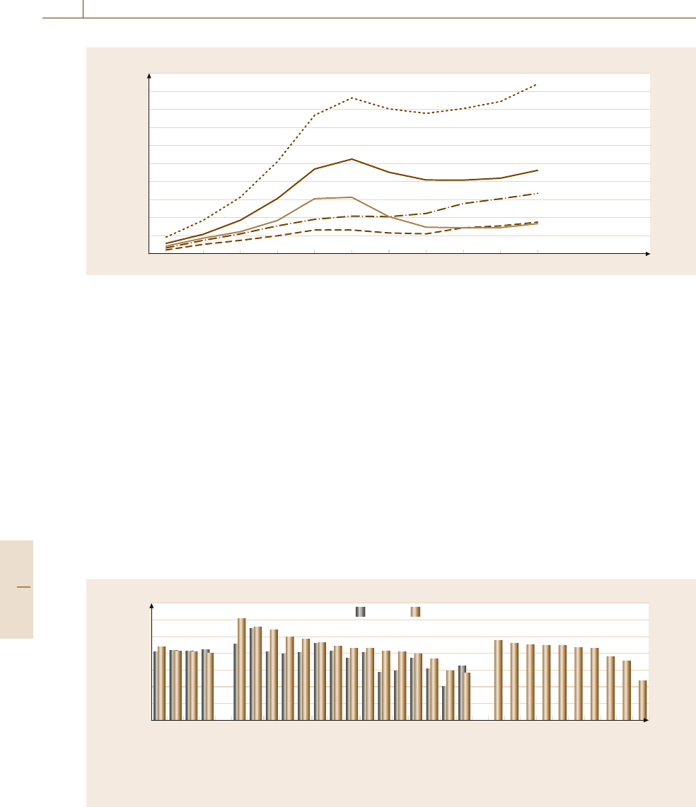
Fig. 6.6 Employment growth by sector with special focus on computer and ICT (source: OECD Information Technology
Outlook 2008, based on STAN database)
should increase automation in order to obtain high uti-
lization of production capacity. One positive effort in
this direction has been the design and implementation
of flexible automation during recent decades (e.g., see
Chap.50 on Flexible and Precision Assembly).
Moving from microeconomic to macroeconomic
considerations, automation should reduce the effects
on short-term inflation caused by nominal salary in-
creases since it forces productivity to augment more
than the markup necessary to cover higher fixed costs.
In addition, the impact of automation depends on the
book-keeping method adoptedby the enterprisein order
to recover the capital value: this impact is lower if a part
of capital can be financed by debts and if the enterprise
behavior is motivated by monetary illusion.
Poland
Turkey
EU15
Australia
Canada
United States
Luxembourg
United Kingdom
Denmark
Finland
Sweden
Netherlands
Italy
Belgium
Germany
Ireland
Austria
France
Spain
Greece
Portugal
Norway
Switzerland
Hungary
Iceland
Czech Republic
Slovenia
Estonia
Slovak Republic
Share (%)
1995 2007
35
30
25
20
15
10
5
0
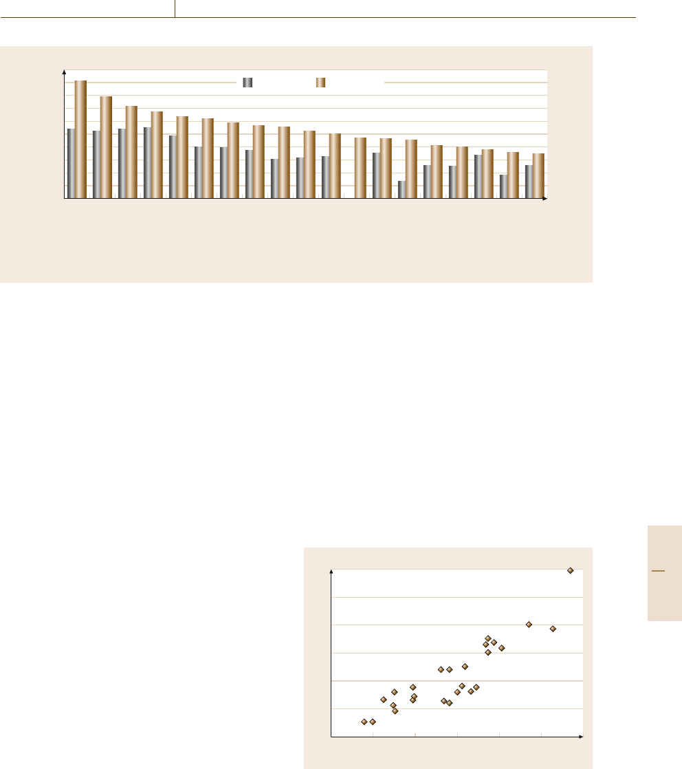
Fig. 6.7 Share of ICT-related occupations in the total economy from 1995 and 2007 (source: OECD IT Outlook 2008,
forthcoming)
Over a mid-term period, automation has been rec-
ognized to have beneficial effects (Figs. 6.6–6.8) both
on the real salary paid to workers and on the (natural)
unemployment trend, if characteristics of automation
technologies donot form an obstacleto the market trend
towards equilibrium, i. e., negotiation between enter-
prises and trade unions. If, on the contrary, the system
production capacity, for a compatible demand, prevents
market convergence, a noncontractual equilibrium only
dependent on technology capability could be estab-
lished, to the advantage of enterprises and the prejudice
of workers, thus reducing real wages and increasing the
unemployment rate.
Empirical validation seems to show that Italy
entered this technology-caused unemployment phase
Part A 6.5
Economic Aspects of Automation 6.6 Capital/Labor and Capital/Product Ratios in the Most Important Italian Industrial Sectors 113
Australia
United States
Sweden
Denmark
United Kingdom
Belgium
Canada
Japan
New Zealand
Spain
Netherlands
Portugal
Finland
Ireland
Greece
Italy
Germany
France
Austria
%
1990–95 1995–2003
1
0.9
0.8
0.7
0.6
0.5
0.4
0.3
0.2
0.1
0
Fig. 6.8 Contributions of ICT investment to GDP growth, 1990–1995 and 1995–2003 in percentage points (source:
OECD Productivity Database, September 2005)
during the last 20 years: this corresponds to a flatter
Phillips curve because absence of inflation acceler-
ation is related to natural unemployment rates that
increase with automation diffusion, even if some struc-
tural modification of the labor market restrained this
trend.
6.6 Capital/Labor and Capital/Product Ratios
in the Most Important Italian Industrial Sectors
A list of the most important industrial sectors in
Italy is reported in Table 6.2 (data collected by
Mediobanca [6.52] for the year 2005). The following
estimations of the model variables and rates have been
adopted (as enforced by the available data): capital K
is estimated through fixed assets; with reference to pro-
duction, the added value V
a
is considered; labor L is
estimated in terms of number of workers.
Some interesting comments can be made based on
Table 6.2, by using the production function models pre-
sented in the previous sections.
According tothe authors’experience (based on their
knowledge of the Italian industrial sectors), the follow-
ing anomalous sectors can be considered:
•
Sectors concerning energy production and distribu-
tion and public services for the following reasons:
they consist of activities applying very high levels
of automation; personnel applied in production are
extremely scarce, whilst it is involved in organiza-
tion and control; therefore anomalous values of the
capital/labor ratio and of productivity result.
•
The transport sector, because the very high capi-
tal/product ratio depends on the low level of the
added value of enterprises that are operating with
politically fixed (low) prices.
0123456
Capital/labor (×1000 Euro)
Capital/production (rate)
600
500
400
300
200
100
0
Fig. 6.9 Correlation between capital/labor (× 1000€)and
capital/production (ratios)
Part A 6.6

114 Part A Development and Impacts of Automation
Table 6.2 Most important industrial sectors in Italy (after [6.52])
Industrial sector Fixedassets Added Number Capital/ Capital/ Productivity
(year 2005) (million value of workers product labor (× 1000
euro) (a) (million (× 1000) (a/b) (× 1000 eu ro) (b/c)
euro) (b) (c) euro) (a/c)
Industrial enterprises 309689.6 84373.4 933.8 3.7 331.6 90.4
Service enterprises 239941.9 42278.3 402.7 5.7 595.8 105.0
Clothing industry 2824.5 1882.9 30.4 1.5 93.0 62.0
Food industry: drink production 5041.7 1356.2 14.3 3.7 352.1 94.7
Food industry: milk & related products 1794.6 933.2 10.1 1.9 177.8 92.5
Food industry: alimentary preservation 2842.4 897.8 11.2 3.2 252.9 79.9
Food industry: confectionary 4316.1 1659.0 17.8 2.6 242.7 93.3
Food industry: others 5772.7 2070.2 23.9 2.8 241.4 86.6
Paper production 7730.9 1470.6 19.9 5.3 388.2 73.9
Chemical sector 16 117.7 4175.2 47.7 3.9 337.7 87.5
Transport means production 21771.4 6353.3 121.8 3.4 178.8 52.2
Retail distribution 10141.1 3639.8 84.2 2.8 120.4 43.2
Electrical household appliances 4534.7 1697.4 35.4 2.7 128.1 47.9
Electronic sector 9498.9 4845.4 65.4 2.0 145.1 74.0
Energy production/distribution 147 200.4 22 916.2 82.4 6.4 1786.8 278.2
Pharmaceuticals & cosmetics 9058.9 6085.2 56.3 1.5 160.8 108.0
Chemical fibers 2081.4 233.2 5.0 8.9 418.4 46.9
Rubber & cables 3868.3 1249.7 21.2 3.1 182.1 58.8
Graphic & editorial 2399.1 1960.4 18.0 1.2 133.3 108.9
Plant installation 1295.9 1683.4 23.2 0.8 56.0 72.7
Building enterprises 1337.7 1380.0 24.7 1.0 54.2 55.9
Wood and furniture 2056.1 689.2 12.8 3.0 160.2 53.7
Mechanical sector 18114.1 9356.6 137.3 1.9 131.9 68.1
Hide and leather articles 1013.9 696.6 9.0 1.5 113.1 77.7
Products for building industry 11585.2 2474.3 28.7 4.7 404.3 86.4
Public services 103 746.7 28 413.0 130.5 3.7 795.2 217.8
Metallurgy 18885.6 5078.2 62.4 3.7 302.9 81.4
Textile 3539.5 1072.1 21.7 3.3 163.2 49.4
Transport 122989.3 7770.5 142.1 15.8 865.2 54.7
Glass 2929.3 726.2 9.2 4.0 317.8 78.8
Notation: Labor-intensive sectors Intermediate Anomalous
•
The chemical fibres sector, because at the time con-
sidered it was suffering a deep crisis with a large
amount of unused production capacity, which gave
rise to an anomalous (too high) capital/product ratio
and anomalous (too small) value of productivity.
Sectors with a rate capital/production of 1.5(such
as the clothing industry, pharmaceutics and cosmet-
ics, and hide and leather articles) has been considered
as intermediate sectors, because automation is highly
important in some working phases, whereas otherwork-
ing phases still largely utilize workers. These sectors
(and the value 1.5 of the rate capital/production) are
used as separators between capital-intensive systems
(with high degrees of automation) and labor-intensive
ones.
Sectors with a capital/production ratio of less than
1.5 have been considered as labor-intensive systems.
Among these, note that the graphic sector is capital in-
tensive, but available data for this sector are combined
with the editorial sector, which in turn is largely labor
intensive.
Part A 6.6
