Nielsen H. RNA: Methods and Protocols

Подождите немного. Документ загружается.

54 Torarinsson

with some more concrete examples to help us ﬁnd information

relevant to the structure of the transcription unit. I r ecommend

that you read this chapter while using a computer to follow the

instructions. In selected sections I have added questions (in the

Notes section) to make this chapter more interactive and to help

you understand the potential of genome browsers.

2. Getting Started

The three major genome browsers at UCSC, Ensembl and NCBI

all provide two main entry points to the browsers. These are with

a known sequence or querying for known coor dinates or some

search term. In this chapter we will focus on the case when we

know which gene we are interested in. If you want to enter the

browsers with an unknown sequence, instead of a known gene,

do not worry, the browser navigation described below is exactly

the same, the only difference is that you use BLAT (UCSC) or

BLAST (Ensembl and NCBI) to compare your sequence to their

database and enter browser via the results, and not by accessing

it directly with a known gene. Beware, although major updates

on the browsers’ appearances are rare, some things might have

changed since this was written.

2.1. UCSC

1. Point your browser to http://genome.ucsc.edu.

2. Choose either “Genomes” or “Genome Browser” in the top

left corner.

3. Here you can choose the clade, the genome, and which

assembly. In the ﬁelds named “position or search term” you

can enter different kinds of information. These include the

following:

– Gene names → BRCA1

– Speciﬁc region → chr7:1–10,000 or simply chr7

– Keywords → kinase, receptor, speciﬁc disease

– IDs → NP, NM, OMIM and more

4. To demonstrate we will use the Human assembly from

March 2006 and search for DTNBP1 (see Fig. 5.1). When

you search for this you get a list of data matching your search

term. In our case I chose the third listing under UCSC genes

Fig. 5.1. How you search for DTNBP1 in the UCSC genome browser.

Genome Browsers 55

“dystrobrevin binding protein 1 isoform a.” By following

this link you will reach the heart of the browser.

2.1.1. Genome Browser

To better understand how this browser works it is good to know

the basic organization of the underlying data. Everything in the

browser is organized along the genomic sequence backbone.

The data exist in so-called “tracks,” which are kept in MySQL

databases. For example, there is a track called “UCSC Genes”

and the corresponding database for this track holds information

like the name and the ID of this gene, which chromosome it

belongs to and start and stop positions (also start positions for

the UTR and exons, etc.). The positions are all relative to the

genomic backbone, so if we are studying a region on chromo-

some 7 between position 10 and 10,000, the genome browser

will check the “UCSC Genes” track and plot a gene on the image

if it ﬁnds an overlap. The tracks are grouped together so that each

group contains similar type of information, i.e., the “Genes and

Gene Prediction Tracks.” Continuing with our DTNBP1 exam-

ple we are now at the heart of the genome browser.

5. If you have never used your current computer to access the

UCSC genome browser it will display the default tracks; oth-

erwise, if you used it before, it will remember if you removed

or added tracks and show these tracks again. If you are inter-

ested in the default tracks, simply click the “default tracks”

button. To begin with all this information can be over-

whelming so we start by removing all the tracks by selecting

the “Hide all” button, located just below the image.

6. Now the image is almost empty, only displaying where we

are on chromosome 6. Now let us add the “UCSC Genes”

track. The “UCSC Genes” track is located under the “Genes

and Gene Prediction Tracks.” By clicking on the pulldown

menu you will usually have ﬁve options:

– “Hide”: completely removes a track from your image.

– “Dense”: all items become collapsed into a single line –

fuses all the rows of data into one.

– “Squish”: each item is on a separate line, but at 50% of its

regular height.

– “Pack”: each item is separate, but efﬁciently stacked like

sardines. However, they are full height, which makes it

different from squish.

– “Full”: each item, e.g., gene, is on a separate line.

By selecting the link above the pulldown menus you can read

the information about the track, how it was generated, and so on.

Sometimes you may further specify how the track should be dis-

played. In the “UCSC Genes” case you can, for example, change

which ID it displays and read that this track is based on Ref-

56 Torarinsson

Seq, UniProt, CCDS, and Comparative Genomics. Let us choose

“full” for the “Known Genes” track. Then we update the image

by clicking on the “Refresh” button, either just below the image

or at the bottom of the page.

7. The image now displays a few versions of the DTNBP1 gene,

with different colors (see Note 2). Our selected isoform is

the one with dark blue background in its name (DTNBP1).

The full-size boxes indicate exons, the half size-boxes indi-

cate UTRs, and the arrows indicate the direction of the tran-

scription.

8. To get mor e information about the gene you click on one

of the genes (see Note 3), (see Note Q-1). This takes you

to a new page with many information and links to other

databases with further details about this gene. On the top

of this page there are links to all the information within this

page, and just below ther e are links to external databases and

other resources within UCSC like the “Proteome Browser”

and “VisiGene.”

9. Finally, it is worth mentioning that when you ar e on the page

with the browser image, there are a couple of useful links on

the top in the blue horizontal bar. Selecting “DNA” will

able you to get the DNA sequence for the region where the

browser is located; furthermore, there are several options to

manipulate the DNA output, like repeats in lower case and

coloring of some features. The “PDF/PS” link gives you a

PDF and a PS-formatted ﬁ le of the image, which is useful

for publications or presentations.

Although we only used two tracks and one genome in this

little example, the beauty of the genome browser is that the pro-

cedure is exactly the same for all the tracks and genomes. The

procedure is always the same but the information available varies

between tracks and genomes. So if you can follow this small exam-

ple, you should be able to study every track and genome in the

browser. The best way to learn to navigate the browser is by exper-

imenting on your own.

2.2. Ensembl

1. Point your browser to http://www.ensembl.org/index.

html.

2. We stay true to our species and select Homo sapiens, assem-

bly GRCh37 (the link to the right next to the “Michelan-

gelo” icon).

3. Here we can search with some search term similar to UCSC.

Here we search for DTNBP1 again. Below “By Species”

click on “Homo sapiens” and then “Gene” to go to the

search results (you can also enter “By Feature type” her e ,

it does not matter).

Genome Browsers 57

4. This gives us two matches, either the Havana or the Ensembl

protein coding gene. We choose Ensembl since it contains

more information. There are two different links, a long one

with the name and a shorter one named “Region in detail.”

The long link will take you directly to gene report for this

gene, whereas the “Region in detail” link will take you to the

Ensemble equivalent of the UCSC genome browser. Let us

start by selecting the “Region in detail.” Like UCSC every-

thing in the viewer is organized along the genomic sequence

backbone in different tracks.

5. This V iew displays three image boxes. The top image titled

“Chromosome 6” shows chromosome 6 with a red box sur-

rounding the region where we are. The next image zooms

in on chromosome 6, again with a red box surrounding

the region where we are. The information in this view

includes “Contigs,” Ensembl/Havana genes, non-coding

RNA (ncRNA) genes, and ncRNA pseudogenes. Here, the

red box surrounds our DTNBP1 gene and we can see that

there is a gene named JARID2 upstream of our gene. Fur-

thermore, the ncRNA gene U6 is upstream of our gene.

Here, we can click on every gene to obtain further infor-

mation about each gene, but before you do that, study the

bottom image.

6. The bottom image is where we can hide and show all the

tracks available at Ensembl. To add or remove tracks, follow

the “Conﬁgure this page” link in the left-side navigation.

You select the group of tracks on the left and click on the

box in front of the track you are interested to select if and

how it should be displayed. Finally, click on the “Save and

Close” icon in the top right corner of the popup window,

this will update the image (see Note 4). If you have a look

at the “Ensembl/Havana gene” track you see that exons are

indicated with ﬁlled boxes and UTRs with non-ﬁlled boxes.

7. In the bottom view, if you click on one of the transcripts

in the “Ensembl/Havana genes” track like the “DTBP1-

001” you will see a popup box. In this box you can choose

between accessing the gene, transcript, or peptide informa-

tion page. Choose the gene (“Gene:ENSG00000047579”).

This will take you to the gene report for that gene.

8. This page displays the usual information at the top like the

ID and a description. Below that, there are some data con-

cerning the transcripts. In the left menu you can ﬁnd links

to features that are often very relevant in understanding

the gene structure and potential regulation of this gene (see

Note Q-2). These will be discussed in more details in the

next section.

58 Torarinsson

3. Comparative

Genomics

UCSC and Ensembl are useful in different ways, when studying

the conservation of a given gene in different organisms. UCSC is

very good to quickly locate highly conserved regions, for exam-

ple, high conservation upstream, downstream, or in the UTR

of a given gene, indicating a possible regulatory role of that

region. With UCSC you can ﬁnd links, from the gene informa-

tion page, to a few orthologues and view them separately in the

browser. Ensembl on the other hand has many more orthologue

predictions, with emphasis on predictions, and it is possible to

view them simultaneously. This makes things like comparing exon

structure and genomic context much easier with Ensembl. Fur-

thermore , it is easy to retrieve pairwise or multiple alignments.

Let us work with an example to illustrate these different strengths.

3.1. UCSC

1. Like in our earlier example, we go to http://genome.

ucsc.edu and choose “Genome Browser” in the top left

corner.

2. In this example we will work with homeobox C8. Select

Human, assembly March 2006, and either search for hoxc8

(and choose the ﬁrst match in “UCSC Genes”) or go directly

to the location “chr12:52,689,157-52,692,812.”

3. To ease the visual inspection of the tracks, start by clicking

on “hide all” tracks just below the image. Now select “pack”

in the pulldown menus for the “UCSC Genes,” “Conser-

vation” and “28-way Most Cons” (see Note 5) tracks (in

the “Comparative Genomics” group). Click on “Refresh”

to apply your changes.

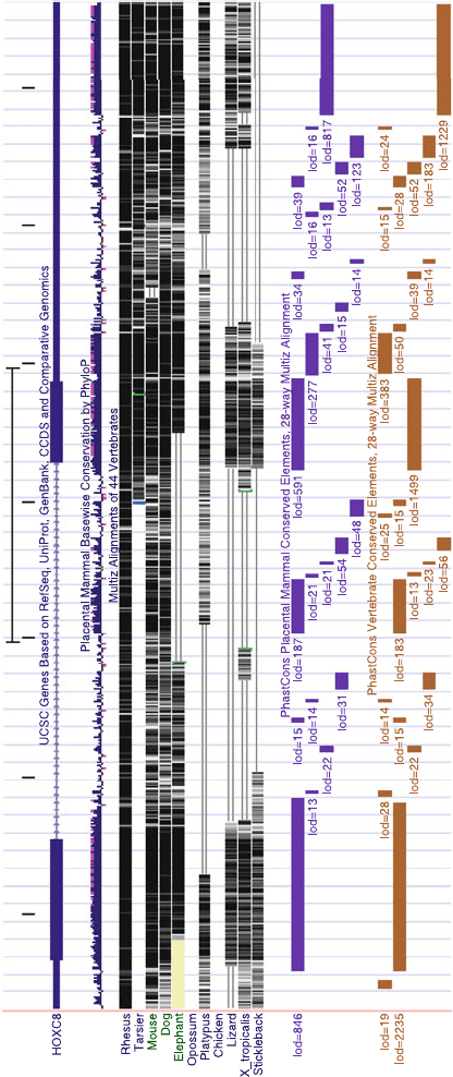
4. The image (see Fig. 5.2) now displays the HOXC8 gene.

Below the “UCSC Genes” track you see the “Conservation”

track. The histogram indicates the level of conservation and

below you can see where the conserved regions lie in the

respective organisms. Finally, at the bottom you see the “28-

way Most Cons” track. It is often interesting to study the

gene and the conservation simultaneously, like for this gene

we can see that the 3



UTR is extremely well conserved. It

is often good to be aware of simple things like this when

studying the transcription and regulation of this gene (see

Note Q-3).

3.2. Ensembl

1. Point your browser to http://www.ensembl.org/index.

html.

2. Select the human genome and then search for HOXC8.

Click on “Homo sapiens” and the “Gene.” Go to the

gene report page for the Ensembl gene (the Ensembl ID is

Genome Browsers 59

Scale

chr12:

1 kb

52689500 52690000 52690500 52691000 52691500 52692000 52692500

Vertebrate Multiz Alignment & Conservation (44 Species)

PhastCons Conserved Elements, 28-way Vertebrate Multiz Alignment

Fig. 5.2. A UCSC genome browser image displaying three tracks, the “UCSC Genes” track, the “Conservation” track, and the “28-way Most Cons” track.

60 Torarinsson

ENSG00000037965). Do NOT click on “Region in detail”

click on the long link with the gene name; this will take you

directly to the gene report page.

3. The gene report for HOXC8 reveals, amongst other things,

that there is only one known transcript, several putative

orthologues, and several putative paralogues in human

(Orthologues and Paralogues links are in the left-side

menu).

4. From the link “Genomic alignments” you can view this

gene in genomic alignments to other species. Select the

“11 eutherian mammals EPO” from the “Select an align-

ment” pulldown. Right click on “Go to a graphical

view” and open it in a new window/tab. This win-

dow makes it quite easy to compare genomic contexts

in several species simultaneously. Now we are at zoom

level two (the bar on the right surrounded by “+” and

“−” icons is at position 2) and only see HOXC8; let

us change to zoom level ﬁve by clicking on bar num-

ber ﬁve (corresponds to region 54354719–54454718) (see

Fig. 5.3).

5. Studying the genomic context of a given gene in sev-

eral organisms can often be very useful. For example,

when studying how the gene might be regulated, but

also to do things like annotate genes. One could say that

it is quite likely that the “Novel RNA genes” ENSB-

TAG00000029788 and ENSECAG00000026361 in cow

and horse, respectively, is the micro RNA miR-196, consid-

ering the annotation in the other mammals. So here we have

a relatively easy way of using well-annotated organisms, to

help annotate other less annotated organisms.

6. Now go back to the gene report for human HOXC8; if you

do not have it open, just go back or click on the HOXC8

gene in the human box. In the Orthologues view you can

do four things: (i) click on the ﬁrst link and view the gene

report for the orthologue, (ii) click on “Multi-species view”

where you can view the orthologue, together with your

gene, in a similar way to what we just did in Step 5, (iii)

click on “Align” to obtain the alignment between your gene

and your orthologue. Via “Conﬁgure this page” you can

choose between DNA or peptide, several output formats,

and species, and (iv) view the gene tree.

7. Still in the Orthologue view, we can click on “View sequence

alignments of these homologues.” As the name implies, this

will show all the pairwise orthologues and paralogues align-

ments (the same as clicking on “Align” for every ortho-

logue).

8. Finally in the transcript view, in accessed through the

“Transcript: HOXC8-201” link at the top (next to “Gene:

Genome Browsers 61

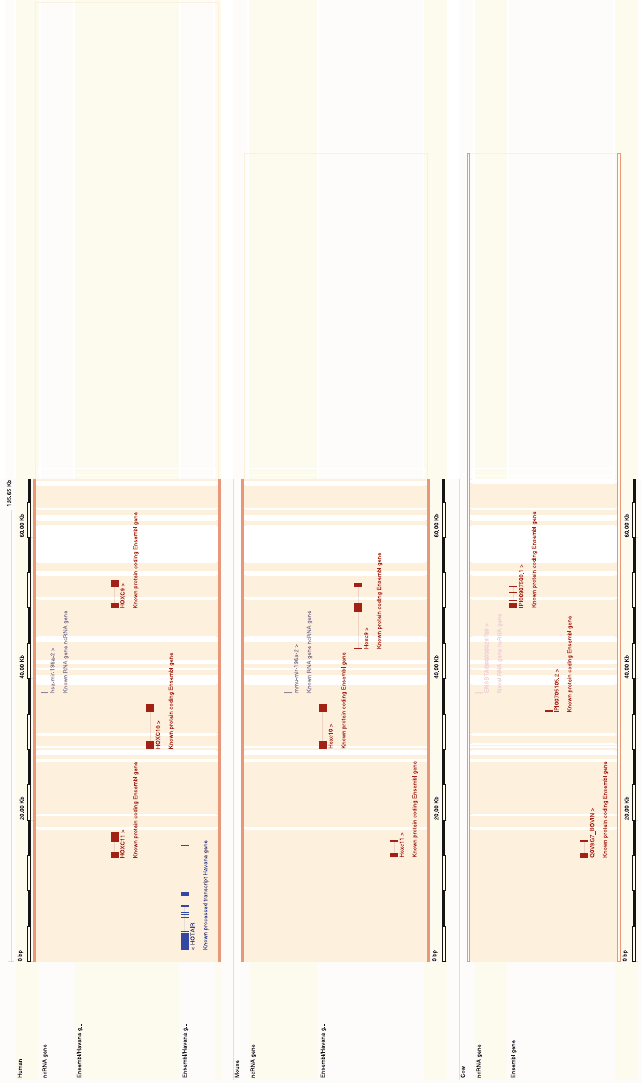
Fig. 5.3. A simpliﬁed image of the region surrounding the HOXC8 gene in humans. This image only shows the Ensembl/Ha vana genes and ncRNAs for human, mouse and cow (i.e.,

in “Conﬁgure this page” I removed some default tracks and species).

62 Torarinsson

HOXC8”) ther e is more interesting data to be obtained.

These include the following links:

– “Gene Ontology”: where you can see which GO terms

(see Note 6) have been mapped to this gene, and by fol-

lowing the links there you can further information con-

cerning the GO term.

– “Domains & features”: where you see which domains the

gene has and view all the genes with the same domain.

– “Population comparison”: where you can see variations in

this transcript (i.e., to Watson and Venter).

4. Expression

and Regulation

Again, when studying expression and regulation, the strengths of

UCSC and Ensembl are different. UCSC, with its simple way of

viewing many tracks simultaneously, makes it very e asy to com-

pare your gene with various expression and regulation tracks. To

some extent this is also possible in Ensembl, though it is mor e dif-

ﬁcult and time consuming. What Ensembl has is a nice view of the

regulatory factors from the cisRED database, predicted miRNA

target sites from miranda analysis, and regulatory features from

the Ensembl Regulatory Build, to mention a few. Again, with

custom tracks, this is also possible in UCSC but more difﬁcult.

Here is a simple example.

4.1. UCSC

1. We continue studying the HOXC8 gene. If you do not have

it open fr om Section 3.1, repeat Steps 1–3.

2. Select “conﬁgure” under the browser image. Scroll down to

the “Expression” and “Regulation” groups, click on “show

all” for both groups and then "submit" at the top of the

page.

3. Here you can compare our gene with several expression

tracks from GNF, Yale and Affymetrix. Regulatory tracks

include, for example, CpG islands, conserved transcription

factor binding sites, regulatory elements from the ORe-

gAnno database, and a track displaying ESPERR regulatory

potential scores computed from alignments of seven organ-

isms (the darker the color, the higher regulatory potential)

(see Note Q-4).

4.2. Ensembl

1. We continue studying the HOXC8 gene. If you do not have

it open fr om Section 3.2, repeat Steps 1 and 2.

Genome Browsers 63

2. In the left menu, select “Regulation.” This page contains

a graphical display and a listing with relevant links of reg-

ulatory features from the cisRED database and regulatory

features from the Ensembl Regulatory Build, among others

(see Note Q-5).

5. Other

I have just covered a fraction of the functionality at UCSC and

Ensembl. There are several other interesting features in both

browsers.

5.1. UCSC

Other interesting features at UCSC include the VisiGene browser

and the ENCODE tracks. The VisiGene browser is a virtual

microscope for viewing in situ images. These images show where

a gene is used in an organism, sometimes down to cellular res-

olution. With VisiGene users can retrieve images that meet spe-

ciﬁc search criteria, then interactively zoom and scroll across the

collection. A link to the VisiGene browser is available from the

UCSC browser home page.

If your gene of interest happens to be located in the

ENCODE regions, there are many ENCODE speciﬁc tracks avail-

able. This r eveals all the ENCODE tracks, which can be viewed

like any other track we have looked at so far. The ENCODE tracks

include groups like “Transcription,” “Chromatin Immunoprecip-

itation,” “Chromatin Structure,” and additional “Comparative

Genomics and Variation” tracks.

5.2. Ensembl

No matter if you are looking at a gene report or the “Region in

detail” many of the most interesting features at Ensembl are often

located in the left menu. For example, when viewing a gene report

you can view a multiple alignment of the genomic sequence with

several organisms, or get a nice graphical phylogenetic tree (the

“Gene Tree (image)” link) or variations (the “Variation table” and

“Variation image” links). The “Variation table” site has a listing

over the variations, where they are, which alleles are involved and

if they are synonymous or non-synonymous when located in a

coding region.

6. Notes

1. Much more detailed information and good online tutorials

are available for the browsers. OpenHelix (http://www.

openhelix.com/downloads/ucsc/ucsc_home.shtml)