Munson B.R. Fundamentals of Fluid Mechanics

Подождите немного. Документ загружается.

Thus, if is the net pressure force on the particle in the streamline direction, it follows that

Note that the actual level of the pressure, p, is not important. What produces a net pressure

force is the fact that the pressure is not constant throughout the fluid. The nonzero pressure gradi-

ent, is what provides a net pressure force on the particle. Viscous forces,

represented by are zero, since the fluid is inviscid.

Thus, the net force acting in the streamline direction on the particle shown in Fig. 3.3 is given by

(3.3)

By combining Eqs. 3.2 and 3.3, we obtain the following equation of motion along the streamline

direction:

(3.4)

We have divided out the common particle volume factor, that appears in both the force and

the acceleration portions of the equation. This is a representation of the fact that it is the fluid den-

sity 1mass per unit volume2, not the mass, per se, of the fluid particle that is important.

The physical interpretation of Eq. 3.4 is that a change in fluid particle speed is accomplished

by the appropriate combination of pressure gradient and particle weight along the streamline. For

fluid static situations this balance between pressure and gravity forces is such that no change in

particle speed is produced—the right-hand side of Eq. 3.4 is zero, and the particle remains sta-

tionary. In a flowing fluid the pressure and weight forces do not necessarily balance—the force

unbalance provides the appropriate acceleration and, hence, particle motion.

dV,

g sin u 

 rV

 ra

 dw

 dF

 ag sin u 

b dV

t ds dy,

§p  0p



0s sˆ  0p



0n nˆ,



ds dn dy 

dV

 1p  dp

dn dy  1p  dp

2 dn dy 2 dp

dn dy

3.2 F ⴝ ma along a Streamline 97

The net pressure

force on a particle

is determined by the

pressure gradient.

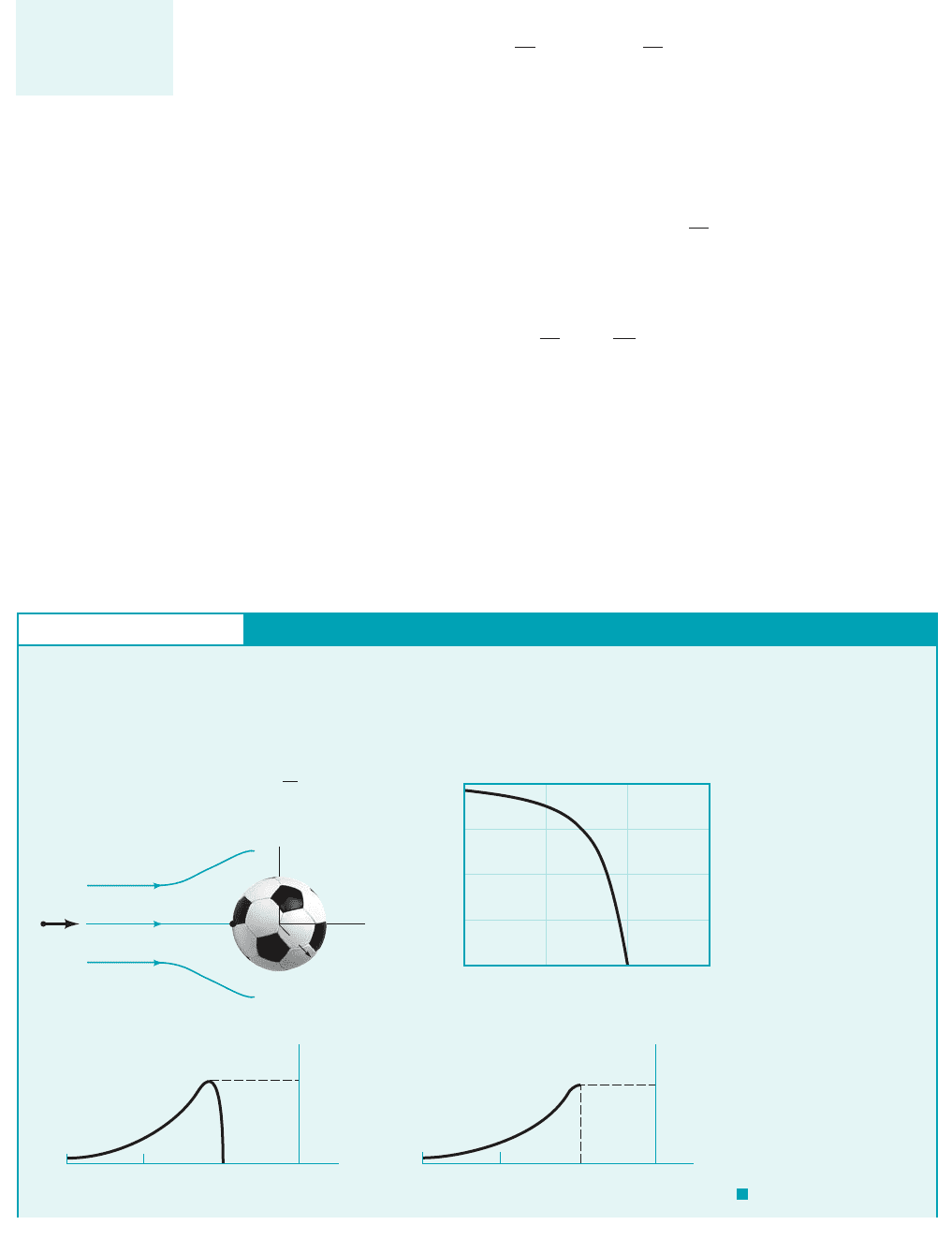
FIND Determine the pressure variation along the streamline

from point A far in front of the sphere and to

point B on the sphere and V

 02.1x

a

 V

21x



Pressure Variation along a Streamline

XAMPLE 3.1

GIVEN Consider the inviscid, incompressible, steady flow

along the horizontal streamline A–B in front of the sphere of ra-

dius a, as shown in Fig. E3.1a. From a more advanced theory of

flow past a sphere, the fluid velocity along this streamline is

as shown in Fig. E3.1b.

V  V

a1 

–3a –2a –a 0

∂p

∂

0.610 V

(c)

–3a –2a –a 0

(d)

0.5 V

= V

= Vi

= 0

(a)

(

–3a –2a –1a 0

0.75

0.5

0.25

F I G U R E E3.1

JWCL068_ch03_093-146.qxd 9/23/08 9:10 AM Page 97

Equation 3.4 can be rearranged and integrated as follows. First, we note from Fig. 3.3 that along

the streamline Also, we can write Finally, along the streamline the

value of n is constant so that Hence, as indi-

cated by the figure in the margin, along a given streamline p(s, n)  p(s) and These

ideas combined with Eq. 3.4 give the following result valid along a streamline

This simplifies to

(3.5)

which, for constant acceleration of gravity, can be integrated to give

(3.6)

where C is a constant of integration to be determined by the conditions at some point on the

streamline.





 gz  C

1along a streamline2

dp 

rd1V

2 g dz  0

1along a streamline2

g





d1V



0s  dp



ds.

10p



0n2 dn  10p



0s2 ds.dp  10p



0s2 ds 1dn  02

V dV



ds 

d1V



ds.sin u  dz



ds.

98 Chapter 3 ■ Elementary Fluid Dynamics—The Bernoulli Equation

OLUTION

This variation is indicated in Fig. E3.1c. It is seen that the pres-

sure increases in the direction of flow from point A

to point B. The maximum pressure gradient occurs

just slightly ahead of the sphere It is the pressure

gradient that slows the fluid down from to as

shown in Fig. E3.1b.

The pressure distribution along the streamline can be obtained

by integrating Eq. 2 from 1gage2at to pressure p at

location x. The result, plotted in Fig. E3.1d,is

(Ans)

COMMENT The pressure at B, a stagnation point since

is the highest pressure along the streamline

As shown in Chapter 9, this excess pressure on the front of the

sphere 1i.e., 2contributes to the net drag force on the

sphere. Note that the pressure gradient and pressure are directly

proportional to the density of the fluid, a representation of the fact

that the fluid inertia is proportional to its mass.

7 0

 rV



22.V

 0,

p rV





x p  0

 0V

 V

1x 1.205a2.

10.610 rV



10p



0x 7 02

Since the flow is steady and inviscid, Eq. 3.4 is valid. In addition,

since the streamline is horizontal, and the

equation of motion along the streamline reduces to

(1)

With the given velocity variation along the streamline, the

acceleration term is

where we have replaced s by x since the two coordinates are iden-

tical 1within an additive constant2along streamline A–B. It follows

that along the streamline. The fluid slows down

from far ahead of the sphere to zero velocity on the “nose” of

the sphere

Thus, according to Eq. 1, to produce the given motion the

pressure gradient along the streamline is

(2)



3ra

11  a



1x a2.

V 0V



0s 6 0

3V

a1 

 V

a1 

b a

rV

sin u  sin 0°  0

Fluids in the News

Incorrect raindrop shape The incorrect representation that

raindrops are teardrop shaped is found nearly everywhere—

from children’s books, to weather maps on the Weather Chan-

nel. About the only time raindrops possess the typical teardrop

shape is when they run down a windowpane. The actual shape

of a falling raindrop is a function of the size of the drop and re-

sults from a balance between surface tension forces and the air

pressure exerted on the falling drop. Small drops with a radius

less than about 0.5 mm are spherical shaped because the sur-

face tension effect (which is inversely proportional to drop

size) wins over the increased pressure, , caused by the

motion of the drop and exerted on its bottom. With increasing

size, the drops fall faster and the increased pressure causes the

drops to flatten. A 2-mm drop, for example, is flattened into a

hamburger bun shape. Slightly larger drops are actually con-

cave on the bottom. When the radius is greater than about

4 mm, the depression of the bottom increases and the drop

takes on the form of an inverted bag with an annular ring of wa-

ter around its base. This ring finally breaks up into smaller

drops. (See Problem 3.28.)



p = p(s)

Streamline

n = constant

For steady, inviscid

flow the sum of cer-

tain pressure, ve-

locity, and

elevation effects is

constant along a

streamline.

JWCL068_ch03_093-146.qxd 8/19/08 10:21 PM Page 98

In general it is not possible to integrate the pressure term because the density may not be con-

stant and, therefore, cannot be removed from under the integral sign. To carry out this integration we

must know specifically how the density varies with pressure. This is not always easily determined.

For example, for a perfect gas the density, pressure, and temperature are related according to

where R is the gas constant. To know how the density varies with pressure, we must also

know the temperature variation. For now we will assume that the density and specific weight are con-

stant 1incompressible flow2. The justification for this assumption and the consequences of compress-

ibility will be considered further in Section 3.8.1 and more fully in Chapter 11.

With the additional assumption that the density remains constant 1a very good assumption

for liquids and also for gases if the speed is “not too high”2, Eq. 3.6 assumes the following sim-

ple representation for steady, inviscid, incompressible flow.

(3.7)

This is the celebrated Bernoulli equation—a very powerful tool in fluid mechanics. In 1738 Daniel

Bernoulli 11700–17822published his Hydrodynamics in which an equivalent of this famous equa-

tion first appeared. To use it correctly we must constantly remember the basic assumptions used

in its derivation: 112viscous effects are assumed negligible, 122the flow is assumed to be steady,

132the flow is assumed to be incompressible, 142the equation is applicable along a streamline. In

the derivation of Eq. 3.7, we assume that the flow takes place in a plane 1the x–z plane2. In gen-

eral, this equation is valid for both planar and nonplanar 1three-dimensional2flows, provided it is

applied along the streamline.

We will provide many examples to illustrate the correct use of the Bernoulli equation and will

show how a violation of the basic assumptions used in the derivation of this equation can lead to

erroneous conclusions. The constant of integration in the Bernoulli equation can be evaluated if suf-

ficient information about the flow is known at one location along the streamline.

p 

 gz  constant along streamline

r  p



RT,

3.2 F ⴝ ma along a Streamline 99

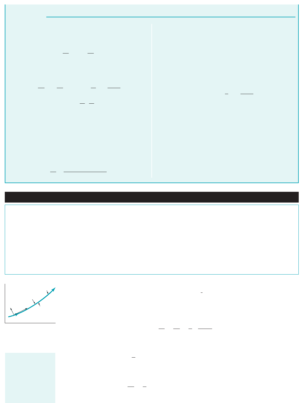
GIVEN Consider the flow of air around a bicyclist moving

through still air with velocity as is shown in Fig. E3.2.

FIND Determine the difference in the pressure between points

112and 122.

OLUTION

The Bernoulli Equation

the velocity distribution along the streamline, was known.

The Bernoulli equation is a general integration of To

determine knowledge of the detailed velocity distri-

bution is not needed—only the “boundary conditions” at 112and

122are required. Of course, knowledge of the value of V along

the streamline is needed to determine the pressure at points

between 112and 122. Note that if we measure we can de-

termine the speed, As discussed in Section 3.5, this is the

principle upon which many velocity measuring devices are

based.

If the bicyclist were accelerating or decelerating, the flow

would be unsteady 1i.e., constant2and the above analysis

would be incorrect since Eq. 3.7 is restricted to steady flow.



 p

F  ma.

V1s2,

XAMPLE 3.2

In a coordinate fixed to the ground, the flow is unsteady as the bi-

cyclist rides by. However, in a coordinate system fixed to the bike,

it appears as though the air is flowing steadily toward the bicyclist

with speed V

. Since use of the Bernoulli equation is restricted to

steady flows, we select the coordinate system fixed to the bike. If

the assumptions of Bernoulli’s equation are valid 1steady, incom-

pressible, inviscid flow2, Eq. 3.7 can be applied as follows along

the streamline that passes through 112and 122

We consider 112to be in the free stream so that and 122to

be at the tip of the bicyclist’s nose and assume that and

1both of which, as is discussed in Section 3.4, are reason-

able assumptions2. It follows that the pressure at 122is greater than

that at 112by an amount

(Ans)

COMMENTS A similar result was obtained in Example 3.1

by integrating the pressure gradient, which was known because

 p



 0

 z

 V



 gz

 p



 gz

= 0

= V

(1)

(2)

F I G U R E E3.2

V3.3 Flow past a

biker

V3.2 Balancing

ball

JWCL068_ch03_093-146.qxd 8/19/08 10:21 PM Page 99

The difference in fluid velocity between two points in a flow field, and can often be

controlled by appropriate geometric constraints of the fluid. For example, a garden hose nozzle

is designed to give a much higher velocity at the exit of the nozzle than at its entrance where it

is attached to the hose. As is shown by the Bernoulli equation, the pressure within the hose must

be larger than that at the exit 1for constant elevation, an increase in velocity requires a decrease

in pressure if Eq. 3.7 is valid2. It is this pressure drop that accelerates the water through the noz-

zle. Similarly, an airfoil is designed so that the fluid velocity over its upper surface is greater 1on

the average2than that along its lower surface. From the Bernoulli equation, therefore, the aver-

age pressure on the lower surface is greater than that on the upper surface. A net upward force,

the lift, results.

100 Chapter 3 ■ Elementary Fluid Dynamics—The Bernoulli Equation

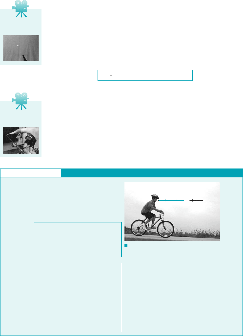
In this section we will consider application of Newton’s second law in a direction normal to

the streamline. In many flows the streamlines are relatively straight, the flow is essentially

one-dimensional, and variations in parameters across streamlines 1in the normal direction2can

often be neglected when compared to the variations along the streamline. However, in nu-

merous other situations valuable information can be obtained from considering normal

to the streamlines. For example, the devastating low-pressure region at the center of a tornado

can be explained by applying Newton’s second law across the nearly circular streamlines of

the tornado.

We again consider the force balance on the fluid particle shown in Fig. 3.3 and the figure in

the margin. This time, however, we consider components in the normal direction, and write New-

ton’s second law in this direction as

(3.8)

where represents the sum of n components of all the forces acting on the particle and

is particle mass. We assume the flow is steady with a normal acceleration where is

the local radius of curvature of the streamlines. This acceleration is produced by the change in di-

rection of the particle’s velocity as it moves along a curved path.

We again assume that the only forces of importance are pressure and gravity. The compo-

nent of the weight 1gravity force2in the normal direction is

If the streamline is vertical at the point of interest, and there is no component of the par-

ticle weight normal to the direction of flow to contribute to its acceleration in that direction.

If the pressure at the center of the particle is p, then its values on the top and bottom of the

particle are and where Thus, if is the net pressure

force on the particle in the normal direction, it follows that

Hence, the net force acting in the normal direction on the particle shown in Fig 3.3 is given by

(3.9)

By combining Eqs. 3.8 and 3.9 and using the fact that along a line normal to the streamline

1see Fig. 3.32, we obtain the following equation of motion along the normal direction

(3.10a)g





cos u  dz



 dw

 dF

 ag cos u 

dV



ds dn dy 

dV

 1p  dp

2 ds dy  1p  dp

2 ds dy 2 dp

ds dy

 10p



0n21dn



22.p  dp

,p  dp

u  90°,

dw cos u g dV cos u

 V



dmg dF



dm V



r dV V

nˆ,

F  ma

3.3 Normal to a Streamline

F ⴝ ma



To apply F  ma

normal to stream-

lines, the normal

components of

force are needed.

V3.4 Hydrocyclone

separator

V3.5 Aircraft wing

tip vortex

JWCL068_ch03_093-146.qxd 8/19/08 10:22 PM Page 100

The physical interpretation of Eq. 3.10 is that a change in the direction of flow of a fluid

particle 1i.e., a curved path, 2is accomplished by the appropriate combination of pressure

gradient and particle weight normal to the streamline. A larger speed or density or a smaller radius

of curvature of the motion requires a larger force unbalance to produce the motion. For example,

if gravity is neglected 1as is commonly done for gas flows2or if the flow is in a horizontal

plane, Eq. 3.10 becomes

(3.10b)

This indicates that the pressure increases with distance away from the center of curvature

1 is negative since is positive—the positive n direction points toward the “inside”

of the curved streamline2. Thus, the pressure outside a tornado 1typical atmospheric pres-

sure2is larger than it is near the center of the tornado 1where an often dangerously low

partial vacuum may occur2. This pressure difference is needed to balance the centrifugal

acceleration associated with the curved streamlines of the fluid motion. (See Fig. E6.6a in

Section 6.5.3.)



r0p





1dz



dn  02

r 6 

3.3 F ⴝ ma Normal to a Streamline 101

Weight and/or pres-

sure can produce

curved streamlines.

V3.6 Free vortex

GIVEN Shown in Figs. E3.3a,b are two flow fields with circu-

lar streamlines. The velocity distributions are

for case (a)

and

for case (b)

where V

is the velocity at

FIND Determine the pressure distributions, p  p(r), for each,

given that p  p

at r  r

r  r

V1r2

V1r2 1V

OLUTION

Pressure Variation Normal to a Streamline

XAMPLE 3.3

F I G U R E E3.3

= ᏾

(a)

V = (V

)r V = (V

(b)

We assume the flows are steady, inviscid, and incompressible

with streamlines in the horizontal plane (dz/dn  0). Because the

streamlines are circles, the coordinate n points in a direction op-

posite that of the radial coordinate, ∂/∂n  ∂/∂r, and the radius

of curvature is given by r  r. Hence, Eq. 3.9 becomes

For case (a) this gives

whereas for case (b) it gives

For either case the pressure increases as r increases since ∂p/∂r  0.

Integration of these equations with respect to r, starting with a

known pressure p  p

at r  r

,gives

(Ans)

p  p

 1␳V



2231r/r

 14



␳1V

 ␳1V



␳V

for case (a) and

(Ans)

for case (b). These pressure distributions are shown in Fig. E3.3c.

COMMENT The pressure distributions needed to balance the

centrifugal accelerations in cases (a) and (b) are not the same be-

cause the velocity distributions are different. In fact, for case (a) the

p  p

 1rV



2231  1r

0 0.5 1 1.5 2 2.5

2

4

6

r/r

(c)

p – p

(b)

(a)

JWCL068_ch03_093-146.qxd 9/23/08 9:10 AM Page 101

If we multiply Eq. 3.10 by dn, use the fact that if s is constant, and integrate

across the streamline 1in the n direction2we obtain

(3.11)

To complete the indicated integrations, we must know how the density varies with pressure and

how the fluid speed and radius of curvature vary with n. For incompressible flow the density is

constant and the integration involving the pressure term gives simply We are still left, how-

ever, with the integration of the second term in Eq. 3.11. Without knowing the n dependence in

and this integration cannot be completed.

Thus, the final form of Newton’s second law applied across the streamlines for steady, in-

viscid, incompressible flow is

(3.12)

As with the Bernoulli equation, we must be careful that the assumptions involved in the derivation

of this equation are not violated when it is used.

p  r



dn  gz  constant across the streamline

r  r1s, n2V  V1s, n2









dn  gz  constant across the streamline



0n  dp



102 Chapter 3 ■ Elementary Fluid Dynamics—The Bernoulli Equation

pressure increases without bound as r → , whereas for case (b)

the pressure approaches a finite value as r → . The streamline

patterns are the same for each case, however.

Physically, case (a) represents rigid body rotation (as obtained

in a can of water on a turntable after it has been “spun up”) and

case (b) represents a free vortex (an approximation to a tornado, a

hurricane, or the swirl of water in a drain, the “bathtub vortex”).

See Fig. E6.6 for an approximation of this type of flow.

In the previous two sections, we developed the basic equations governing fluid motion under a

fairly stringent set of restrictions. In spite of the numerous assumptions imposed on these flows,

a variety of flows can be readily analyzed with them. A physical interpretation of the equations

will be of help in understanding the processes involved. To this end, we rewrite Eqs. 3.7 and 3.12

here and interpret them physically. Application of along and normal to the streamline re-

sults in

(3.13)

and

(3.14)

as indicated by the figure in the margin.

The following basic assumptions were made to obtain these equations: The flow is steady

and the fluid is inviscid and incompressible. In practice none of these assumptions is exactly

true.

A violation of one or more of the above assumptions is a common cause for obtaining an

incorrect match between the “real world” and solutions obtained by use of the Bernoulli equa-

tion. Fortunately, many “real-world” situations are adequately modeled by the use of Eqs. 3.13

and 3.14 because the flow is nearly steady and incompressible and the fluid behaves as if it were

nearly inviscid.

The Bernoulli equation was obtained by integration of the equation of motion along the “nat-

ural” coordinate direction of the streamline. To produce an acceleration, there must be an unbalance

of the resultant forces, of which only pressure and gravity were considered to be important. Thus,

p  r



dn  gz  constant across the streamline

p 

 gz  constant along the streamline

F  ma

3.4 Physical Interpretation

The sum of pres-

sure, elevation, and

velocity effects is

constant across

streamlines.

p + r



dn +

= constant



p + r

= constant

JWCL068_ch03_093-146.qxd 8/19/08 10:22 PM Page 102

there are three processes involved in the flow—mass times acceleration 1the term2, pressure

1the p term2, and weight 1the term2.

Integration of the equation of motion to give Eq. 3.13 actually corresponds to the work-

energy principle often used in the study of dynamics [see any standard dynamics text 1Ref. 12].

This principle results from a general integration of the equations of motion for an object in a way

very similar to that done for the fluid particle in Section 3.2. With certain assumptions, a statement

of the work-energy principle may be written as follows:

The work done on a particle by all forces acting on the particle is equal to the change

of the kinetic energy of the particle.

The Bernoulli equation is a mathematical statement of this principle.

As the fluid particle moves, both gravity and pressure forces do work on the particle. Recall

that the work done by a force is equal to the product of the distance the particle travels times the

component of force in the direction of travel 1i.e., 2. The terms and p in Eq. 3.13

are related to the work done by the weight and pressure forces, respectively. The remaining term,

is obviously related to the kinetic energy of the particle. In fact, an alternate method of de-

riving the Bernoulli equation is to use the first and second laws of thermodynamics 1the energy

and entropy equations2, rather than Newton’s second law. With the appropriate restrictions, the gen-

eral energy equation reduces to the Bernoulli equation. This approach is discussed in Section 5.4.

An alternate but equivalent form of the Bernoulli equation is obtained by dividing each term

of Eq. 3.7 by the specific weight, to obtain

Each of the terms in this equation has the units of energy per weight or length 1feet,

meters2and represents a certain type of head.

The elevation term, z, is related to the potential energy of the particle and is called the eleva-

tion head. The pressure term, is called the pressure head and represents the height of a column

of the fluid that is needed to produce the pressure p. The velocity term, is the velocity head

and represents the vertical distance needed for the fluid to fall freely 1neglecting friction2if it is to

reach velocity V from rest. The Bernoulli equation states that the sum of the pressure head, the ve-

locity head, and the elevation head is constant along a streamline.



2g,



1LF



F  L2



 z  constant on a streamline



gzwork  F ⴢ d



3.4 Physical Interpretation 103

The Bernoulli

equation can be

written in terms of

heights called

heads.

GIVEN Consider the flow of water from the syringe shown in

Fig. E3.4(a). As indicated in Fig. E3.4b, a force, F, applied to the

plunger will produce a pressure greater than atmospheric at point

112within the syringe. The water flows from the needle, point 122,

with relatively high velocity and coasts up to point 132at the top of

its trajectory.

FIND Discuss the energy of the fluid at points 112, 122, and 132by

using the Bernoulli equation.

Kinetic, Potential, and Pressure Energy

XAMPLE 3.4

Energy Type

Kinetic Potential Pressure

Point p

1 Small Zero Large

2 Large Small Zero

3 Zero Large Zero



(1)

(2)

(3)

(b)

F I G U R E E3.4

(a)

JWCL068_ch03_093-146.qxd 8/19/08 10:22 PM Page 103

A net force is required to accelerate any mass. For steady flow the acceleration can be in-

terpreted as arising from two distinct occurrences—a change in speed along the streamline and

a change in direction if the streamline is not straight. Integration of the equation of motion along

the streamline accounts for the change in speed 1kinetic energy change2and results in the Bernoulli

equation. Integration of the equation of motion normal to the streamline accounts for the cen-

trifugal acceleration and results in Eq. 3.14.

When a fluid particle travels along a curved path, a net force directed toward the center of cur-

vature is required. Under the assumptions valid for Eq. 3.14, this force may be either gravity or pres-

sure, or a combination of both. In many instances the streamlines are nearly straight so that

centrifugal effects are negligible and the pressure variation across the streamlines is merely hydro-

static 1because of gravity alone2, even though the fluid is in motion.

1r 2



104 Chapter 3 ■ Elementary Fluid Dynamics—The Bernoulli Equation

If the assumptions 1steady, inviscid, incompressible flow2of the

Bernoulli equation are approximately valid, it then follows that

the flow can be explained in terms of the partition of the total en-

ergy of the water. According to Eq. 3.13 the sum of the three types

of energy 1kinetic, potential, and pressure2or heads 1velocity, ele-

vation, and pressure2must remain constant. The table above indi-

cates the relative magnitude of each of these energies at the three

points shown in the figure.

The motion results in 1or is due to2a change in the magnitude

of each type of energy as the fluid flows from one location to an-

other. An alternate way to consider this flow is as follows. The

pressure gradient between 112and 122produces an acceleration to

eject the water from the needle. Gravity acting on the particle be-

tween 122and 132produces a deceleration to cause the water to

come to a momentary stop at the top of its flight.

COMMENT If friction 1viscous2effects were important,

there would be an energy loss between 112and 132and for the given

the water would not be able to reach the height indicated in the

figure. Such friction may arise in the needle 1see Chapter 8 on

pipe flow2or between the water stream and the surrounding air

1see Chapter 9 on external flow2.

OLUTION

Fluids in the News

Armed with a water jet for huntingArcherfish, known for their

ability to shoot down insects resting on foliage, are like subma-

rine water pistols. With their snout sticking out of the water, they

eject a high-speed water jet at their prey, knocking it onto the wa-

ter surface where they snare it for their meal. The barrel of their

water pistol is formed by placing their tongue against a groove in

the roof of their mouth to form a tube. By snapping shut their

gills, water is forced through the tube and directed with the tip of

their tongue. The archerfish can produce a pressure head within

their gills large enough so that the jet can reach 2 to 3 m. How-

ever, it is accurate to only about 1 m. Recent research has shown

that archerfish are very adept at calculating where their prey will

fall. Within 100 milliseconds (a reaction time twice as fast as a

human’s), the fish has extracted all the information needed to pre-

dict the point where the prey will hit the water. Without further vi-

sual cues it charges directly to that point. (See Problem 3.41.)

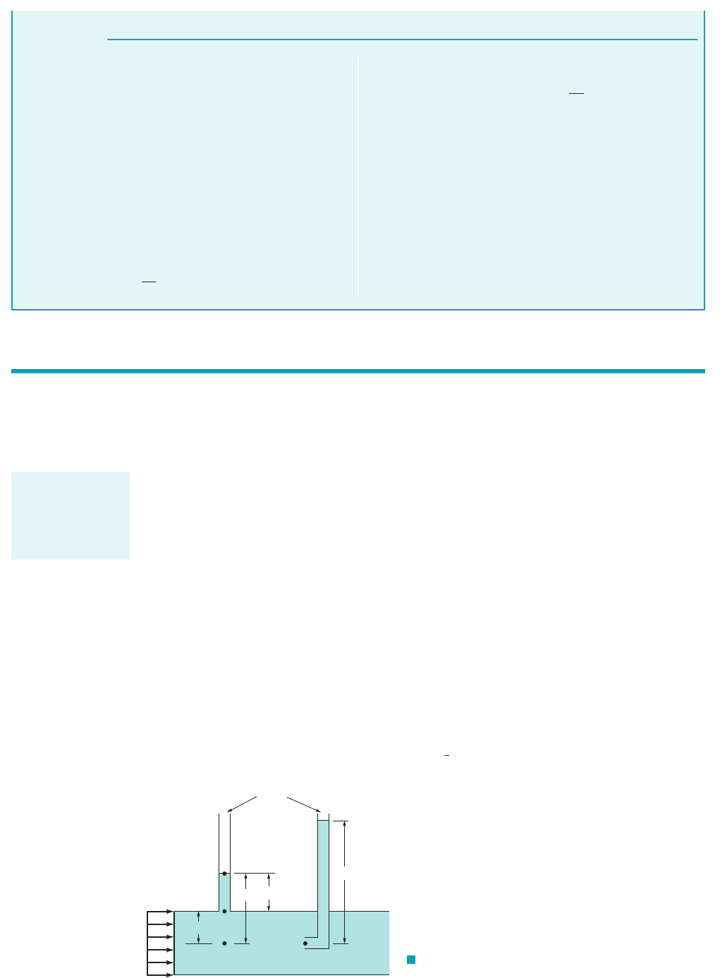
GIVEN Water flows in a curved, undulating waterslide as

shown in Fig. E3.5a. As an approximation to this flow, consider

Pressure Variation in a Flowing Stream

XAMPLE 3.5

(2)

(1)

2-1



Free surface

(

p = 0)

4-3

(4)

(3)

F I G U R E E3.5

(Photo courtesy of

Schlitterbahn

Waterparks.)

The pressure varia-

tion across straight

streamlines is hy-

drostatic.

the inviscid, incompressible, steady flow shown in Fig. E3.5b.

From section A to B the streamlines are straight, while from C to D

they follow circular paths.

FIND Describe the pressure variation between points 112and 122

and points 132and 142.

JWCL068_ch03_093-146.qxd 8/19/08 10:22 PM Page 104

3.5 Static, Stagnation, Dynamic, and Total Pressure 105

With the above assumptions and the fact that for the por-

tion from A to B, Eq. 3.14 becomes

The constant can be determined by evaluating the known variables at

the two locations using and to give

(Ans)

Note that since the radius of curvature of the streamline is infinite,

the pressure variation in the vertical direction is the same as if the

fluid were stationary.

However, if we apply Eq. 3.14 between points 132and 142we ob-

tain 1using 2

 r



1dz2 gz

 p

 gz

dn dz

 p

 g1z

 z

2 p

 gh

2–1

 h

2–1

 0 1gage2, z

 0,

p  gz  constant

r 

With and this becomes

(Ans)

To evaluate the integral, we must know the variation of V and

with z. Even without this detailed information we note that the in-

tegral has a positive value. Thus, the pressure at 132is less than the

hydrostatic value, by an amount equal to

This lower pressure, caused by the curved streamline, is neces-

sary to accelerate the fluid around the curved path.

COMMENT Note that we did not apply the Bernoulli equa-

tion 1Eq. 3.132across the streamlines from 112to 122or 132to 142.

Rather we used Eq. 3.14. As is discussed in Section 3.8, applica-

tion of the Bernoulli equation across streamlines 1rather than

along them2may lead to serious errors.





r2 dz.gh

4–3

 gh

4–3

 r



 z

 h

4–3

 0

OLUTION

A useful concept associated with the Bernoulli equation deals with the stagnation and dynamic pres-

sures. These pressures arise from the conversion of kinetic energy in a flowing fluid into a “pres-

sure rise” as the fluid is brought to rest 1as in Example 3.22. In this section we explore various results

of this process. Each term of the Bernoulli equation, Eq. 3.13, has the dimensions of force per unit

area—psi, The first term, p, is the actual thermodynamic pressure of the fluid as it

flows. To measure its value, one could move along with the fluid, thus being “static” relative to the

moving fluid. Hence, it is normally termed the static pressure. Another way to measure the static

pressure would be to drill a hole in a flat surface and fasten a piezometer tube as indicated by the

location of point 132in Fig. 3.4. As we saw in Example 3.5, the pressure in the flowing fluid at 112

is the same as if the fluid were static. From the manometer considerations of Chap-

ter 2, we know that Thus, since it follows that

The third term in Eq. 3.13, is termed the hydrostatic pressure, in obvious regard to the hy-

drostatic pressure variation discussed in Chapter 2. It is not actually a pressure but does represent the

change in pressure possible due to potential energy variations of the fluid as a result of elevation changes.

The second term in the Bernoulli equation, is termed the dynamic pressure. Its in-

terpretation can be seen in Fig. 3.4 by considering the pressure at the end of a small tube inserted

into the flow and pointing upstream. After the initial transient motion has died out, the liquid will

fill the tube to a height of H as shown. The fluid in the tube, including that at its tip, 122, will be

stationary. That is, or point 122is a stagnation point.

If we apply the Bernoulli equation between points 112and 122, using and assuming

that we find that

 p



 z

 0

 0,



gz,

 gh.h

3–1

 h

4–3

 hp

 gh

4–3

 gh

3–1

 p



, N



3.5 Static, Stagnation, Dynamic, and Total Pressure

Each term in the

Bernoulli equation

can be interpreted

as a form of pres-

sure.

F I G U R E 3.4 Measurement

of static and stagnation pressures.

(1)

(2)

(3)

(4)

3-1

4-3

Open

= VV

= 0

JWCL068_ch03_093-146.qxd 8/19/08 10:22 PM Page 105

106 Chapter 3 ■ Elementary Fluid Dynamics—The Bernoulli Equation

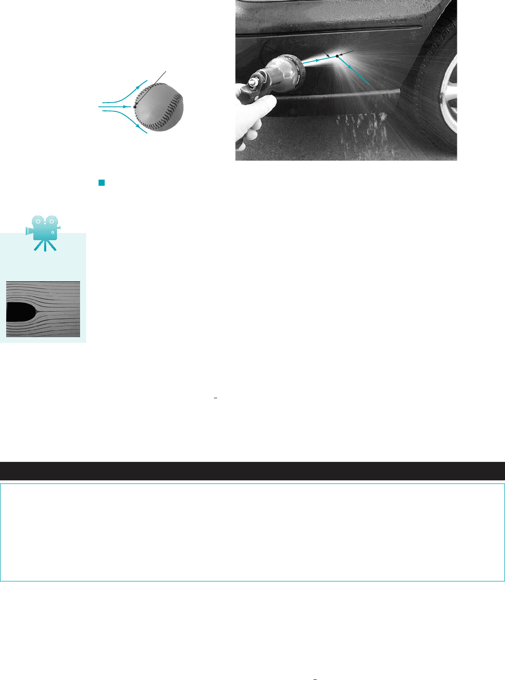
V3.7 Stagnation

point flow

Sta

nation

oint

(

)

Stagnation streamline

(

Stagnation point

F I G U R E 3.5 Stagnation points.

Hence, the pressure at the stagnation point is greater than the static pressure, by an amount

the dynamic pressure.

It can be shown that there is a stagnation point on any stationary body that is placed into a

flowing fluid. Some of the fluid flows “over” and some “under” the object. The dividing line 1or sur-

face for two-dimensional flows2is termed the stagnation streamline and terminates at the stagnation

point on the body. 1See the photograph at the beginning of Chapter 3.2For symmetrical objects 1such

as a baseball2the stagnation point is clearly at the tip or front of the object as shown in Fig. 3.5a.

For other flows such as a water jet against a car as shown in Fig. 3.5b, there is also a stagnation point

on the car.

If elevation effects are neglected, the stagnation pressure, is the largest pressure

obtainable along a given streamline. It represents the conversion of all of the kinetic energy into a

pressure rise. The sum of the static pressure, hydrostatic pressure, and dynamic pressure is termed

the total pressure, The Bernoulli equation is a statement that the total pressure remains con-

stant along a streamline. That is,

(3.15)

Again, we must be careful that the assumptions used in the derivation of this equation are appro-

priate for the flow being considered.

p 

 gz  p

 constant along a streamline

p  rV



Fluids in the News

Pressurized eyes Our eyes need a certain amount of internal pres-

sure in order to work properly, with the normal range being be-

tween 10 and 20 mm of mercury. The pressure is determined by a

balance between the fluid entering and leaving the eye. If the

pressure is above the normal level, damage may occur to the op-

tic nerve where it leaves the eye, leading to a loss of the visual

field termed glaucoma. Measurement of the pressure within the

eye can be done by several different noninvasive types of instru-

ments, all of which measure the slight deformation of the eyeball

when a force is put on it. Some methods use a physical probe that

makes contact with the front of the eye, applies a known force,

and measures the deformation. One noncontact method uses a

calibrated “puff” of air that is blown against the eye. The stagna-

tion pressure resulting from the air blowing against the eyeball

causes a slight deformation, the magnitude of which is correlated

with the pressure within the eyeball. (See Problem 3.29.)

Knowledge of the values of the static and stagnation pressures in a fluid implies that the fluid

speed can be calculated. This is the principle on which the Pitot-static tube is based [H. de Pitot

(1695–1771)]. As shown in Fig. 3.6, two concentric tubes are attached to two pressure gages 1or a

differential gage2so that the values of and 1or the difference 2can be determined. The

center tube measures the stagnation pressure at its open tip. If elevation changes are negligible,

 p 

 p

JWCL068_ch03_093-146.qxd 8/19/08 10:23 PM Page 106