Mei C., Zhou J., Peng X. Simulation and Optimization of Furnaces and Kilns for Nonferrous Metallurgical Engineering
Подождите немного. Документ загружается.


5 Hologram Simulation of Aluminum Reduction Cells
is the “Joule heat”. It can be solved from the Laplace equation of electrical
conduction, i.e. Eq. 5.3.
Eq. 5.52 and the electrical conduction equation can be solved with the implicit
finite difference format after the discretization. For a selected slice, except that the
collector bar is treated as a three-dimensional part, others are all regarded as
two-dimensional. The boundary conditions are the same as stated in Section 5.4.1.
The solving and analysis of the unsteady heat conduction equation are based on
“heat balance self-checking method”(Zuo, 1996). The procedure is:
a) According to the static analytic method, to determine a basic heat balance of
the aluminum cell under a given melt temperature.
b) Supposing that a disturbance will bring the heat to increase
0
QΔ in one
time step and make the melt temperature increase to WQTT /
001
Δ+= (W is the
“water equivalent” of the melt). Under these conditions, the electric field and
temperature field at next moment can be analyzed.
c) To estimate the volume of melted ledge, meanwhile, check the heat balance
and the melt temperature, then start the calculation of next time step.
Melting or freezing of the ledge will result in changes of its edge position,
which can be determined by the “moving boundary method”(You,1997). Take the
melting of the ledge as an example. When disturbances starts and the calculated
temperature of the boundary node exceeds
f
T , the extra enthalpy
H
Δ was
considered to melt the ledge in the control volume around the node. The melted
volume is
λ
H
G
Δ
=Δ
. With the melted volume, a new position of the ledge can
be decided. After several time steps, if the entire ledge in control volume of this
node all melts, the boundary should move to the next node in next step of the
computation. The same computation should be carried out at each node. After
several time steps (which is set as the simulation time in the programme), the
results of the freeze profile of the cell can be obtained and displayed on a
WINDOWS interface. For the process that the ledge freezes and gets thicker, the
computation is the same only the boundary moves in a reverse direction.
As the computation goes on, error will accumulate, thus result in a distortion of
the simulation results. It can be solved by periodically correcting the basic heat
balance offline with the measured electrolyze temperature and freeze profile. Or it
can be done by online correction with the cell wall temperatures (Zhou et al., 1998).
5.5.3
Technical scheme of the dynamic simulation and function
of the software system
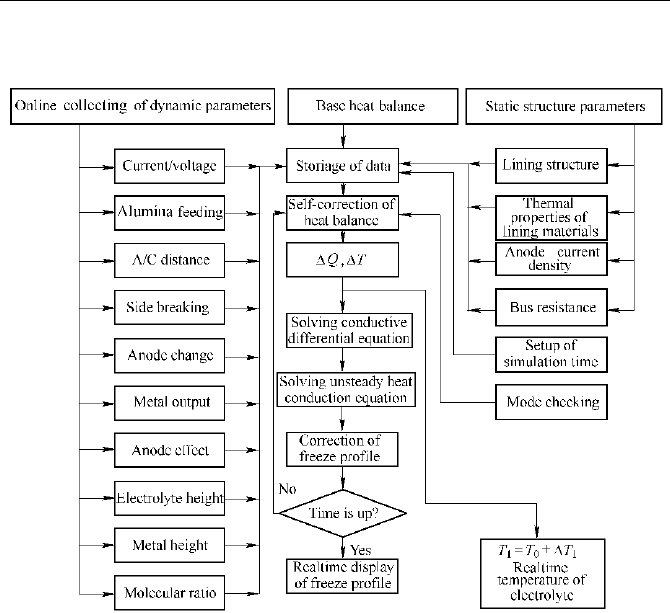
According to above principles and models, in reference (Mei et al.,1998), the author
put forward a technical scheme of the dynamic simulation (as shown in Fig. 5.26).
The software system consists of six function modules, i.e., analysis of cell
conditions, dynamic simulation, examination and correction of static parameters,
Naijun Zhou
offline calibration, creation and print of report forms, and online help. The main
functions of the system are listed below:
Fig. 5.26
Technique scheme of dynamic simulation (Mei et al., 1998)
a) Display of main parameters collected online (such as series current, voltage
and wall temperatures etc.).
b) Display of the graph of simulated freeze profile, and displaying temperature
distribution of the cathode cross section.
c) Display of the dynamic forecasted temperature of the electrolyte and the
molten aluminum.
d) Display of the simulated characteristic dimensions of the freeze profile.
e) Examination and modification of the static structure parameters and physical
parameters.
f) Input and browse of the processing parameters offline.
g) Recording and browse of the operation history.
h) Indication and warning of the communication state.
i) Creation, browse and output of report forms.
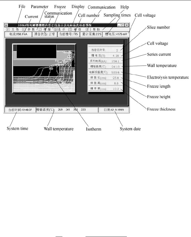
Fig. 5.27 shows an displaying interface of the software. Application of the
software in a 160kA prebaked anode cell were reported in references (Mei et al.,
1997; Mei et al., 1998; Zhou et al., 1998).
5 Hologram Simulation of Aluminum Reduction Cells
Fig. 5.27
Simulation software run in visualization windows and results
(zhou et al., 1998)
For the precision of the simulation, error of electrolyte temperature is estimated
to be less than 0.3
%, and the ledge characteristic dimension is within 10%.
The realtime response of the simulation has been tested, of which the analysis
time of every slice is less than 5s at a P
Ċ300 micro computer. The result indicates
the software has good engineering practical value.
5.6
Model of Current Efficiency of Aluminum Reduction Cells
Current efficiency
η
in an aluminum reduction cell is defined as the percentage
of actual aluminum production to its theoretical production, that is:
at
3
t
100% 100%
0.3356 10
QQ
Q
It
η
−
=× = ×
×
••
(5.53)
where
a
Q is the actual aluminum production of a cell;
t
Q is the theoretical
production of the cell;
I is the current intensity; t is time. There are two kinds of
current efficiency: the “mean current efficiency for a long time” and the “transient
current efficiency”.
The current efficiency in electrolysis aluminum factories in China ranges from
87% to 92%. The advanced international index is about 94% to 95%, and the best
record of tested cells approaches to 96%. The economic benefit resulting from
every 1% increase of the current efficiency is that, not only the production can
increase 1% corresponding, but also the power consumption will reduce 170kW·h

Naijun Zhou
per ton aluminum. Study of the current efficiency has always been a topic of
research of aluminum electrolysis technology since the Hall-Heroult aluminum
reduction method was applied in industry. As a results, the current efficiency
increased from original 60% to the present level, which reflected the great
progress achieved in the aluminum electrolysis technology.
The study of the current efficiency focuses on several aspects, such as the
mechanism of reduction of the current efficiency, the factors influencing current
efficiency, mathematical models of current efficiency and related factors, and
measurements of current efficiency. The research method is mainly experimental
methods including laboratory experiments and industrial experiments. Theoretical
methods are also used in the studies. Theoretical methods usually make some
simplification of various conditions and influencing factors with known theory
and experiences; then on the basis of the process control steps, to deduce a
calculation formula of the current efficiency according to fluid dynamic principles.
The calculation formula, to some extent, simulates the relation among various
factors and the current efficiency, and reflects a good correlation with actual
measurements of the current efficiency. Hence it is proved to be applicable. This
is also the point to be discussed in this section.
5.6.1
Factors influencing current efficiency and its measurements
According to research up to now, the reasons of the reduction of the current
efficiency in aluminum cells come from four aspects (Qiu, 1988; Huang et al.,
1994):
a) Dissolution of the aluminum. The precipitated aluminum dissolves back into
the electrolyte, being brought to the space below anode by the circulating
electrolyte and oxidized by anode gas. This is the main reason for the reduction of
the current efficiency.
b) Precipitation of sodium. The low concentration of alumina and the high
temperature of cell, especially during the anode effect period, will result in sodium
ions replacing with aluminum ions to discharge in the cathode, thus reduce the
productivity of aluminum.
c) Vain consumption of current. It includes vain consumption of current that
caused by imperfect charge of polyvalent ions, electronic conduction, short circuit,
current leakage and so on.
d) Other losses. They include combination reaction of aluminum and inner
lining materials, electrolysis of moisture content and impurity compounds,
mechanical losses in aluminum discharging process and so on.
The effects of various process parameters on current efficiency are summed up
as follows:

5 Hologram Simulation of Aluminum Reduction Cells
a) Temperature. All the research results indicate that increasing of the
temperature causes reduction of current efficiency; and experimental results show
that the current efficiency decreases about 2% when the electrolysis temperature
rise 10
ć.
b) Anode-cathode distance (ACD). The characteristics of the effects of the ACD
on current efficiency are that, the current efficiency improves with increasing of
the ACDs, whereas high ACD will result in higher energy consumption perton
aluminum. Therefore it is not a feasible way to improve the current efficiency by
enlarging ACD.
c) Molecular ratio. No consistent conclusion has been reached about the effects
of the electrolyte molecular ratio on the current efficiency. Results of most
research indicated that the current efficiency decreases with the molecular ratio.
However, low molecular ratio can have impacts on electrolytic conductivity,
solubility and volatilization loss, which should be considered synthetically.
d) Alumina concentration. Research results indicated that there is an optimum
alumina concentration. Exceeding or bellowing alumina concentration will all
decrease the current efficiency. The optimum concentration value depends on the
electrolyte composition.
e) Chemical additives. Lots of experiments have been carried out on the
electrolyte additives. The chemical additives with good influencing performance
include CaF
2
, MgF
2
, Li
2
CO
3
and so on. The action of the additives is mainly to
decrease the electrolysis temperature and to control the dissolution of aluminum,
so that the current efficiency can be improved. Proper amount of the chemical
additive ranges from 3% to 5%. Too much or too less is unfavorable.
f) Area current density. The influence of the area current density includes two
aspects. One is that the current efficiency decreases with the anode area current
density; and the other is the current efficiency increases with the cathode area
current density. However, as the area current density cannot be changed easily
during the operation of cells, it is generally taken into account only in the design.
g) Melt motion. The melt motion strengthens the mass transfer process, thus
accelerates the aluminum dissolution, and it may also cause current short circuit,
which will decrease the current efficiency.
In a word, there are many factors that have influences on the current efficiency.
These factors interrelate with each other, and should not be isolated. As their
effects depends on the control of test conditions, it is difficult to quantify their
respective influences.
There are two main measurements of the current efficiency: the dilution method
and the eudiometry. The dilution method is to put known indicators (such as Cu, Mn,
Ti,
60
Co) into a cell and trace the variation of indicator concentration, thus to calculate
out the current efficiency during this period. Or it also can be done by calculating the
aluminum weight in the cell between two additions of the indicator into the cell. The

Naijun Zhou
current efficiency can then be calculated through adding up and measuring the
tapping aluminum quantity and power consumption in the period. The first method is
called as the regression method, and the latter is the inventory method. The
eudiometry is to calculate the current efficiency with the continuously measured CO
2
concentration in the anode gas using an appropriate formula. Both methods have their
own advantages and disadvantages, and they are often used by combine in utilization.
5.6.2
Models of the current efficiency
The aim of developing a current efficiency model is to express quantitatively the
relationship of parameters and the current efficiency with a mathematical formula,
so as to provide a basis for the computer control of aluminum reduction cells.
There are two methods to establish a current efficiency model. One is to make
theoretical deductions with the reduction mechanism of the current efficiency. The
other is to establish the model through regressing massive experimental data. The
former reflects the internal connection of various parameters to some extents and
has a certain physical meaning, however it is not well practical. The latter is a
empirical formula, however, lacking of clear physical meaning, it is only
applicable in some cases. A lot of research has been carried out on the calculation
of the current efficiency. Here it is to list several representative models.
5.6.2.1
Theoretical model of the current efficiency
To illuminate the general method of theoretical modeling, a deduction is to be
made of the relationship of the current efficiency, the area current density
m
AI ,
the ACD
L and the concentration of metal ions in the anode region
3
C
by using
the diffusion theory. Assumptions made in the model are as follows:
a) The reduction of the current efficiency is caused completely by the metal
aluminum solving into the electrolyte in form of Al
+
and diffusing into the anode
region where it is oxidized as Al
3+
. Effects of the electron transfer and the
convective mass transfer are neglected in the model.
b) Diffusion coefficient of Al
+
and Al
3+
are constants.
c) The concentration of Al
3+
at the cathode surface is certain value.
d) At the beginning of electrolysis, the Al
3+
concentration at the cathode surface
is an equilibrium concentration, and that at the electrolyte surface is zero.
e) Concentrations are allowed to be replaced with ionic activities with the unit
of mol/cm
3
.
f) Consumption and supplement of raw materials are close to a balance.
The metal deposition reaction at the cathode is:
Al3eAl
3
==+
+
(5.54)
The metal solution reaction is:

5 Hologram Simulation of Aluminum Reduction Cells
++
==+ Al3AlAl2
3
(5.55)
Supposing that,
0
C is the aluminum concentration at the cathode surface;
1
C is
the Al
+
concentration, the equilibrium constant in Eq. 5.55 is
0
3
1
C
C
K
= , then:
11
3
33
100
CKCbC==• (5.56)
If the solubility of aluminum in the electrolyte can be expressed as:
3
1
0
bCaS += (5.57)
And when diffusing into the anodes, the oxidation of Al
+
into Al
3+
in the anode region is:
3
Al 2e Al
++
−== (5.58)
Supposing reactions of Eq.5.57 and Eq. 5.58 are a quick process and it is
controlled by diffusion, then, in accordance with the first Fick’s law, the rate of
metal losses from unit of the cathode surface to the anode is:
L
SD
L
SD
V
11
loss
)0(
=
−
= (5.59)
where
1
D is the diffusion coefficient of Al
+
.
And the metal formation rate is:
L
CCD
V
)(
033
formation
−
=
(5.60)
where
3
D
is the diffusion coefficient of Al
3+
;
3
C is the Al
3+
concentration in the
anode region. As the aluminum concentration at the cathode surface
0
C is difficult
to determine, it can be converted into a function of the area current density.
Since:
30
e3
m
CC
I
ND
AL
−
=
•• (5.61)
It can be rewritten as:
03
me33
1
IL
CC
A
NDC
⎛⎞
=−
⎜⎟
⎝⎠
•
••
(5.62)
where
N
e
is the charge per gram ion.
Then the current efficiency can be simply calculated as:
formation loss
formation
1
3
e1m
3
me3
100%
100 100 %
VV
V
NDA
IL
abC
IL A N D
η
−
=×
⎡⎤
⎛⎞
⎢⎥
=− + −
⎜⎟
⎢⎥
⎝⎠
⎣⎦
••
••
••
(5.63)
Although in this formula, effects of temperature and electrolyte character on the
current efficiency are not definitely indicated, and the convection is neglected,
variables
1
D
,
3
D
, a and b are all related to these factors. Through analysis
of the relationship, various formulas of the current efficiency have been obtained,

Naijun Zhou
Several influential models are introduced below.
a) Robl
formula (Robl et al., 1977):
m
1100%
r
r
η
⎛⎞
=− ×
⎜⎟
⎝⎠
(5.64)
where
m
r
and r are respectively the metal formation rate and mass transfer rate
in the electrolyte. Because factors influencing
m
r are complicated and difficult to
be determined, the model is not practical. However, many researchers put forward
their own models on the basis of it.
b) Lillebuen formula (Lillebuen et al.,1980):
)1(3.219100
*
m
5.1
e
17.083.0
e
5.0
e
67.0
mm
1
fCLuDAI −−=
−−−
ρμη
(5.65)
where
I is the current intensity, kA;
m
A is the surface area of the molten
aluminum, m
2
;
m
D is the diffusion coefficient of the metal, m
2
/s;
e
μ
is the
electrolyte viscosity, Pa·s;
e
u is the relative velocity of the electrolyte to the
molten aluminum, m/s; L is the anode-cathode distance, m;
e
ρ
is the density of
the electrolyte, kg/m
3
;
*
m
C is the mass concentration of the metal in the
electrolyte, %; f is the saturation fraction of aluminum at the interface of the
electrolyte and the molten aluminum. Comparatively, parameters in this formula
are easier to be determined, hence, it is used widely.
c) Evans formula (Evans et al., 1981):
Evans put forward his formula on the basis of Robl’s formula as:
0.5
*
me t
mm
DV
rC
ρ
σ
⎛⎞
=
⎜⎟
⎝⎠
(5.66)
where
5.0
t
kV = is the pulsating component of the turbulent velocity; k is the
turbulent kinetic energy; and
σ
is the surface tension coefficiency of the
interface of the molten aluminum and the electrolyte.
In addition, by considering two-dimensional turbulent mass transfer, Shen
Hongyuan et al proposed a model, of which parameters are also easy to be
determined (for details, please refer to reference (Shen et al., 1992)). All the
models mentioned above are supported by themselves’ experimental results.
5.6.2.2
Statistic model of the current efficiency
Qiu Zhuxian et al (Qiu, 1998; Qiu et al., 1981) studied the relations of CO
2
concentration in the anode gas and operating parameters in a 135kA prebaked anode
cell with side processing and central feeding with automatic breaking shells. Using
stepwise regression method, they obtained the following mathematic model:
3252
543141
2
23212
1341.05951.0
2013.009552.01169.0
2183.0304.12.12267.892.1297%CO
XXXX
XXXXXX
XXXX
+
−++
−−−−−=
(5.67)
where
1
X ,
2
X ,
3
X ,
4
X ,
5
X denote respectively deviations of the anode current

5 Hologram Simulation of Aluminum Reduction Cells
distribution (i.e. ADN value), the concentration of alumina, the electrolysis
temperature, the electrolyte height, the concentration of additives (CaF
2
and
MgF
2
), and the molecular ratio. The current efficiency can then be obtained by
choosing appropriate gas equation, such as:
%5.3%)100%CO(
2
1
2
++=
η
(5.68)
Cai Qifeng et al. (Cai et al.,1991)obtained the current efficiency of a 160kA
four risers prebaked anode cell with the multiple regression method:
8765
43212
5105.212.30845591.06148.0
6392.41133.05204.0337.06.392%CO
XXXX
XXXX
++−
+−+−−=
(5.69)
where
1
X ,
2
X ,
3
X ,
4
X ,
5
X ,
6
X ,
7
X ,
8
X are respectively the electrolyte
temperature t
e
, the molten aluminum height, the molecular ratio, the concentration
of alumina, and the concentration of the additives (CaF
2
, MgF
2
and LiF). Checked
by t verification step by step, a optimum regression equation can be obtained,
which is:
%LiF4289.33301.0025.376%CO
e2
+−= t (5.70)
Wang Hua and Wang Huazhang et al obtained their current efficiency models
of 60kA side stud cells and 24kA self-baking cells in similar way, of which detail
are given in references(Wang,1993;Wang et al.,1982). It should be noted that,
present statistic models of the current efficiency are not universal, because they
are usually based on a certain kind of aluminum reduction cells.
References
Aparotsev B A (1998) Simulation for the carbon-cathode of aluminum electrolysis cells.
Non-Ferrous Metals (in Russian), (1): 73
Arai K, Ramazaki K (1975) Heat balance and thermal losses in advanced prebaked anode
cells.
Light Metals, (1): 193
Arita, Ikenouchi (1983) Image of electrolyte and metal convection in aluminum reduction
cells and numerical computation of the interface shape (in Japanese).
Light Metals
(Japan)
, (11)
Cai Qifeng et al (1991) Mathematic model of current efficiency in 160kA central charging
four terminals pre-baked cells (in Chinese).
Light Metals, (5): 25
Cai Qifeng, Mei Chi et al (1993) Calibration experiment and industrial practice of molten
velocity measurement by iron rod method (in Chinese).
Light Metals, (9): 29
Cao Guofa (1991) Three dimensional numerical computation of potential fall in anode (in
Chinese).
Messages of Aluminum & Magnesium, (3): 1
Central South Institute of Mining and Metallurgy (1977)
Reference Data of Nonferrous
Metallurgical Furnace
(in Chinese),Č

Naijun Zhou
Chen Shiyu et al (1986) Computation of current field in aluminum reduction cells with use
of relative electrical parameters (in Chinese). In:
Aluminum Reduction Cells Thesis
Collection of Aluminum Reduction Cells “Three fields”
, 9: 55
Chen Shiyu et al (1987) Mathematic model of magnetic field in aluminum reduction cells
and error analysis (in Chinese).
Journal of Huazhong Institute of Technology, (6): 85
Dekopov U D et al (1978)
Non-Ferrous Metals (in Russian),(1):32
Derneded D (1975) Gas induced circulation in an aluminum reduction cell.
Light Metals,
(1): 111
Evans J W et al (1981) A mathematical model for prediction of currents, magnetic fields,
melt Velocities, melt topography and current efficiency in Hall-Heroult cells.
Metal.
Trans
.: 353
Jean Frederic, Tony Lelievre, Claude LE (2002) Metal pad roll instabilities.
Light Metal:
483~487
Fuzzy Control Research Institute of North China University of Technology (1997)
Development and extension of new control system for aluminum reduction cells (in
Chinese).
Journal of North China University of Technology, 9 (3): 85
Gan Yiren, Zhang Hong (1998) Impervious heat insulation material for aluminum reduction
cells (in Chinese).
Light Metals, (Supplement): 173
Gerbeau J F, Lelievre T et al (2003) Simulations of MHD flows with moving interfaces.
Journal of Computational Physics
,184(1): 163~191
Guo Jianjin (2007) Review of China’s aluminum market in 2006 (in Chinese).
Shanghai
Non-Ferrous Metals
, 28(3)
Haruhiko Ikenouchi et al (1978)
Light Metals, (1): 59
Haupin W E (1971) Calculating thickness of containing walls frozen from melt.
J. METALS.
23(7): 41~44
Haupin W E (1990) The 9th International Course of Process Metallurgy of Aluminum,
Tronheim
Huang Qianrui (2007) Status, problems and development: bauxite resource and aluminum
industry in China (in Chinese).
Conservation and Utilization of Mineral Resources, 3
Huang Yongzhong et al (1994) Production of Aluminum Electrolysis (in Chinese).
Central
South University of Technology Press
, Changsha, 197
Huang Zhaolin et al (1994) Numerical simulation of turbulent flow and melt topography in
aluminum reduction cells (in Chinese).
Computational Physics, 11(2): 179
Imery Buiza J (1989) Electromagnetic optimization of the V-350 cell.
Light Metals, 211
Japan Light Metals Research Institute (1980)
Three Fields Computation Analysis Program
(Internal Data) (in Chinese)
Li Guohua et al (1993) Computation of magnetic field in aluminum reduction cells with use
of double scalar potential method (in Chinese).
Nonferrous Metal, 45(4): 55
Liang Xuemin et al (1998) Mathematic model of physical field in aluminum reduction cells
and computer simulation (in Chinese).
Light Metals, (Supplement): 145
Lillebuen B et al (1980) Variations of side lining temperature, anode position and