Mavko G., Mukerji T., Dvorkin J. The Rock Physics Handbook

Подождите немного. Документ загружается.

The inverse of the Hilbert transform is itself the Hilbert transform with a change

of sign:

f ðxÞ¼

1

ðx

Þdx

 x

f ðxÞ¼ 



F

The analytic signal associated with a real function, f(t), is the complex function

SðtÞ¼f ðtÞiF

ðtÞ

As discussed below, the Fourier transform of S(t) is zero for negative frequencies.

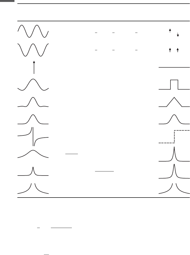
Table 1.1.3 Some Fourier transform pairs.

sin px

d s þ



 d s 



cos px

d s þ



þ d s 



d(x)1

sinc(x) (s)

sinc

(x) L(s)

–px

–ps

–1/pxisgn(s)

þ x

p exp(–2px

jsj)

–jxj

1 þð2psÞ

jxj

–1/2

jsj

–1/2

7 1.2 The Hilbert transform and analytic signal

The instantaneous envelope of the analytic signal is

EðtÞ¼

ﬃﬃﬃﬃﬃﬃﬃﬃﬃﬃﬃﬃﬃﬃﬃﬃﬃﬃﬃﬃﬃﬃﬃﬃﬃﬃﬃ

ðtÞþF

ðtÞ

The instantaneous phase of the analytic signal is

’ðtÞ¼tan

1

½F

ðtÞ=f ðtÞ

¼ Im½lnðSðtÞÞ

The instantaneous frequency of the analytic signal is

o ¼

d’

¼ Im

lnðSÞ



¼ Im



Claerbout (1992) has suggested that o can be numerically more stable if the

denominator is rationalized and the functions are locally smoothed, as in the following

equation:



o ¼ Im



ðtÞ

dSðtÞ



ðtÞSðtÞ

where 〈·〉 indicates some form of running average or smoothing.

Causality

The impulse response, I(t), of a real physical system must be causal, that is,

IðtÞ¼0; for t < 0

The Fourier transform T( f ) of the impulse response of a causal system is some-

times called the transfer function:

Tðf Þ¼

1

IðtÞe

i2pft

T( f ) must have the property that the real and imaginary parts are Hilbert transform

pairs, that is, T( f ) will have the form

Tðf Þ¼Gðf ÞþiBðf Þ

where B( f ) is the Hilbert transform of G( f ):

Bðf Þ¼

1

Gðf

Þdf

 f

Gðf Þ¼

1

Bðf

Þdf

 f

8 Basic tools

Similarly, if we reverse the domains, an analytic signal of the form

SðtÞ¼f ðtÞiF

ðtÞ

must have a Fourier transform that is zero for negative frequencies. In fact, one con-

venient way to implement the Hilbert transform of a real function is by performing the

following steps:

(1) Take the Fourier transform.

(2) Multiply the Fourier transform by zero for f < 0.

(3) Multiply the Fourier transform by 2 for f > 0.

(4) If done numerically, leave the samples at f ¼0 and the Nyquist frequency unchanged.

(5) Take the inverse Fourier transform.

The imaginary part of the result will be the negative Hilbert transform of the real part.

1.3 Statistics and probability

Synopsis

The sample mean, m, of a set of n data points, x

, is the arithmetic average of the data

values:

m ¼

i¼1

The median is the midpoint of the observed values if they are arranged in increasing

order. The sample variance, s

, is the average squared difference of the observed

values from the mean:



i¼1

ðx

 mÞ

(An unbiased estimate of the population variance is often found by dividing the sum

given above by (n – 1) instead of by n.)

The standard deviation, s, is the square root of the variance, while the coefficient

of variation is s/m. The mean deviation, a,is

a ¼

i¼1

 mj

Regression

When trying to determine whether two different data variables, x and y, are related,

we often estimate the correlation coefficient, r, given by (e.g., Young, 1962)

 ¼

i¼1

ðx

 m

Þðy

 m



; where jj1

9 1.3 Statistics and probability

where s

and s

are the standard deviations of the two distributions and m

and m

are their means. The correlation coefficient gives a measure of how close the points

come to falling along a straight line in a scatter plot of x versus y. jrj¼1 if the points

lie perfectly along a line, and jrj< 1 if there is scatter about the line. The numerator

of this expression is the sample covariance, C

, which is defined as

i¼1

ðx

 m

Þðy

 m

It is important to remember that the correlation coefficient is a measure of the linear

relation between x and y. If they are related in a nonlinear way, the correlation

coefficient will be misleadingly small.

The simplest recipe for estimating the linear relation between two variables, x and y,

is linear regression, in which we assume a relation of the form:

y ¼ ax þ b

The coefficients that provide the best fit to the measured values of y, in the least-

squares sense, are

a ¼ 



; b ¼ m

 am

More explicitly,

a ¼



ðÞ



ðÞ

; slope

b ¼

ðÞ





ðÞ



ðÞ

; intercept

The scatter or variation of y-values around the regression line can be described by

the sum of the squared errors as

i¼1

ðy



where

is the value predicted from the regression line. This can be expressed as a

variance around the regression line as

^

i¼1

ðy



The square of the correlation coefficient r is the coefficient of determination, often

denoted by r

, which is a measure of the regression variance relative to the total

variance in the variable y, expressed as

10 Basic tools

¼ 

¼1 

variance of y around the linear regression

total variance of y

¼1 

i¼1

ðy



i¼1

ðy

 m

¼ 1 

^



The inverse relation is

^

¼ 

ð1  r

Often, when doing a linear regression the choice of dependent and independent

variables is arbitrary. The form above treats x as independent and exact and assigns

errors to y. It often makes just as much sense to reverse their roles, and we can find

a regression of the form

x ¼ a

y þ b

Generally a 6¼ 1/a

unless the data are perfectly correlated. In fact, the correlation

coefficient, r, can be written as  ¼

ﬃﬃﬃﬃﬃﬃ

The coefficients of the linear regression among three variables of the form

z ¼ a þ bx þ cy

are given by

b ¼

 C

c ¼

 C

a ¼ m

 m

b  m

The coefficients of the n-dimensional linear regression of the form

z ¼ c

þ c

þþc

are given by

¼ M



1

1ðÞ

2ðÞ

kðÞ

where the k sets of independent variables form columns 2:(n þ 1) in the matrix M:

M ¼

1 x

1ðÞ

 x

1ðÞ

1 x

2ðÞ

 x

2ðÞ

1 x

kðÞ

 x

kðÞ

11 1.3 Statistics and probability

Variogram and covariance function

In geostatistics, variables are modeled as random fields, X(u), where u is the spatial

position vector. Spatial correlation between two random fields X(u) and Y(u)is

described by the cross-covariance function C

(h), defined by

ðhÞ¼Ef½X ðu Þm

ðuÞ½Yðu þ hÞm

ðu þ hÞg

where E{ } denotes the expectation operator, m

and m

are the means of X and Y,andh is

called the lag vector. For stationary fields, m

and m

are independent of position. When

X and Y are the same function, the equation represents the auto-covariance function

(h). A closely related measure of two-point spatial variability is the semivariogram,

g(h). For stationary random fields X(u)andY(u), the cross-variogram 2g

(h) is defined as

ðhÞ¼Ef½X ðu þ hÞXðuÞ½Yðu þ hÞYðuÞg

When X and Y are the same, the equation represents the variogram of X(h). For

a stationary random field, the variogram and covariance function are related by

ðhÞ¼C

ð0ÞC

ðhÞ

where C

(0) is the stationary variance of X.

Distributions

A population of n elements possesses



(pronounced “n choose r”) different

subpopulations of size r  n, where



nðÞ

nn 1ð Þ n  r þ 1ðÞ

1  2  r  1ðÞr

r!ðn  rÞ!

Expressions of this kind are called binomial coefficients. Another way to say this is

that a subset of r elements can be chosen in



different ways from the original set.

The binomial distribution gives the probability of n successes in N independent

trials, if p is the probability of success in any one trial. The binomial distribution is

given by

N; p

ðnÞ¼



ð1  pÞ

Nn

The mean of the binomial distribution is given by

¼ Np

and the variance of the binomial distribution is given by



¼ Npð1  pÞ

12 Basic tools

The Poisson distribution is the limit of the binomial distribution as N !1and

p ! 0 so that l ¼Np remains finite. The Poisson distribution is given by

nðÞ¼

l

The Poisson distribution is a discrete probability distribution and expresses the

probability of n events occurring during a given interval of time if the events have an

average (positive real) rate l, and the events are independent of the time since the

previous event. n is a non-negative integer.

The mean of the Poisson distribution is given by

¼ l

and the variance of the Poisson distribution is given by



¼ l

The uniform distribution is given by

f ðxÞ¼

b  a

; a  x  b

0; elsewhere

The mean of the uniform distribution is

m ¼

ða þ bÞ

and the standard deviation of the uniform distribution is

 ¼

jb  aj

ﬃﬃﬃﬃﬃ

The Gaussian or normal distribution is given by

f ðxÞ¼



ﬃﬃﬃﬃﬃﬃ

ðxmÞ

=2

where s is the standard deviation and m is the mean. The mean deviation for the

Gaussian distribution is

a ¼ 

ﬃﬃﬃ

When m measurements are made of n quantities, the situation is described by the

n-dimensional multivariate Gaussian probability density function (pdf):

ðxÞ¼

ð2pÞ

n=2

jCj

1=2

exp 

ðx  mÞ

1

ðx  mÞ



13 1.3 Statistics and probability

where x

¼(x

, x

,...,x

) is the vector of observations, m

¼(m

, m

,...,m

) is the

vector of means of the individual distributions, and C is the covariance matrix:

C ¼½C



where the individual covariances, C

, are as defined above. Notice that this reduces to

the single variable normal distribution when n ¼1.

When the natural logarithm of a variable, x ¼ln(y), is normally distributed, it

belongs to a lognormal distribution expressed as

f ðyÞ¼

ﬃﬃﬃﬃﬃﬃ

exp 

lnðyÞa



where a is the mean and b

is the variance. The relations among the arithmetic and

logarithmic parameters are

m ¼ e

aþb

; a ¼ lnðmÞb



¼ m

ðe

 1Þ; b

¼ ln 1 þ 



The truncated exponential distribution is given by

PðxÞ¼

expðx=XÞ; x  0

0; x < 0

(

The mean m and variance s

of the exponential distribution are given by

m ¼ X



¼ X

The truncated exponential distribution and the Poisson distribution are closely

related. Many random events in nature are described by the Poisson distribution. For

example, in a well log, consider that the occurrence of a flooding surface is a random

event. Then in every interval of log of length D, the probability of finding exactly

n flooding surfaces is

l D

nðÞ¼

l DðÞ

exp l DðÞ

The mean number of occurrences is lD, where l is the mean number of occurrences

per unit length. The mean thickness between events is D= lDðÞ¼1=l. The interval

thicknesses d between flooding events are governed by the truncated exponential

PðdÞ¼

l expðldÞ; x  0

0; x < 0



the mean of which is 1/l.

14 Basic tools

The logistic distribution is a continuous distribution with probability density

function given by

PxðÞ¼

 xmðÞ=s

s 1 þ e

 xmðÞ=s

½

sech

x  m



The mean m and variance s

of the logistic distribution are given by

m ¼m



The Weibull distribution is a continuous distribution with probability density

function

PðxÞ¼



k1

 x=lðÞ

; x  0

0; x < 0

(

where k > 0istheshape parameter and l > 0isthescale parameter for the distribution.

The mean m and variance s

of the logistic distribution are given by

m ¼l 1 þ





¼l

 1 þ



 m

where G is the gamma function. The Weibull distribution is often used to describe

failure rates. If the failure rate decreases over time, k < 1; if the failure rate is constant

k ¼1; and if the failure rate increases over time, k > 1. When k ¼3, the Weibull

distribution is a good approximation to the normal distribution, and when k ¼1, the

Weibull distribution reduces to the exponential distribution.

Monte Carlo simulations

Statistical simulation is a powerful numerical method for tackling many probabilistic

problems. One of the steps is to draw samples X

from a desired probability distribu-

tion function F(x). This procedure is often called Monte Carlo simulation, a term

made popular by physicists working on the bomb during the Second World War.

In general, Monte Carlo simulation can be a very difficult problem, especially when

X is multivariate with correlated components, and F(x) is a complicated function.

For the simple case of a univariate X and a completely known F(x) (either analytically

or numerically), drawing X

amounts to first drawing uniform random variates

between 0 and 1, and then evaluating the inverse of the desired cumulative distribution

function (CDF) at these U

: X

¼F

–1

). The inverse of the CDF is called the quantile

function. When F

1

(X) is not known analytically, the inversion can be easily done by

15 1.3 Statistics and probability

table-lookup and interpolation from the numerically evaluated or nonparametric CDF

derived from data. A graphical description of univariate Monte Carlo simulation is

shown in Figure 1.3.1.

Many modern computer packages have random number generators not only for

uniform and normal (Gaussian) distributions, but also for a large number of well-known,

analytically defined statistical distributions.

Often Monte Carlo simulations require simulating correlated random variables

(e.g., V

, V

). Correlated random variables may be simulated sequentially, making

use of the chain rule of probability, which expresses the joint probability density in

terms of the conditional and marginal densities: P(V

, V

) ¼P(V

) P(V

A simple procedure for correlated Monte Carlo draws is as follows:



draw a V

sample from the V

distribution;



compute a V

from the drawn V

and the V

–V

regression;



add to the computed V

a random Gaussian error with zero mean and variance equal

to the variance of the residuals from the V

–V

regression.

This gives a random, correlated (V

, V

) sample. A better approach is to draw V

from

the conditional distributions of V

for each given V

value, instead of using a simple

–V

regression. Given sufficient V

–V

training data, the conditional distributions

of V

for different V

can be computed.

Bootstrap

“Bootstrap” is a very powerful computational statistical method for assigning measures

of accuracy to statistical estimates (e.g., Efron and Tibshirani, 1993). The general idea

is to make multiple replicates of the data by drawing from the original data with

replacement. Each of the bootstrap data replicates has the same number of samples

as the original data set, but since they are drawn with replacement, some of the data

may be represented more than once in the replicate data sets, while others might be

0.2

0.4

0.6

0.8

5101520

CDF F(X)

Uniform [0 1]

random number

Simulated X

Figure 1.3.1 Schematic of a univariate Monte Carlo simulation.

16 Basic tools