Massoud M. Engineering Thermofluids: Thermodynamics, Fluid Mechanics, and Heat Transfer
Подождите немного. Документ загружается.

582 IVd. Heat Transfer: Thermal Radiation
(a) (b)
r
1
r
2
A
2
A
1
L
R
1
= r
1
/r
2
R
2
= L/r
2
∞=
2
R
F
21
F
22
F
21
∞=
2
R
F
22
R
1
(c) (d)
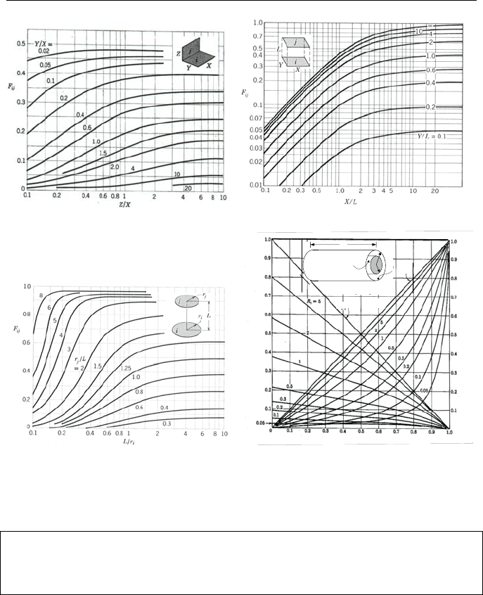
Figure IVd.5.2. Radiation view factor between (a) perpendicular rectangles with a com-
mon edge, (b) parallel rectangles, (c) parallel concentric disks, and (d) coaxial cylinders
Example IVd.5.2. Find the view factor for two parallel rectangles with X = 20 ft,
Y = 40.0 ft, and L = 10 ft.
Solution: Since Y/L = 4 and X/L = 2 from Figure IVd.5.2(a) we find F
ij
≈ 0.52.
5. Radiation Exchange Between Surfaces 583
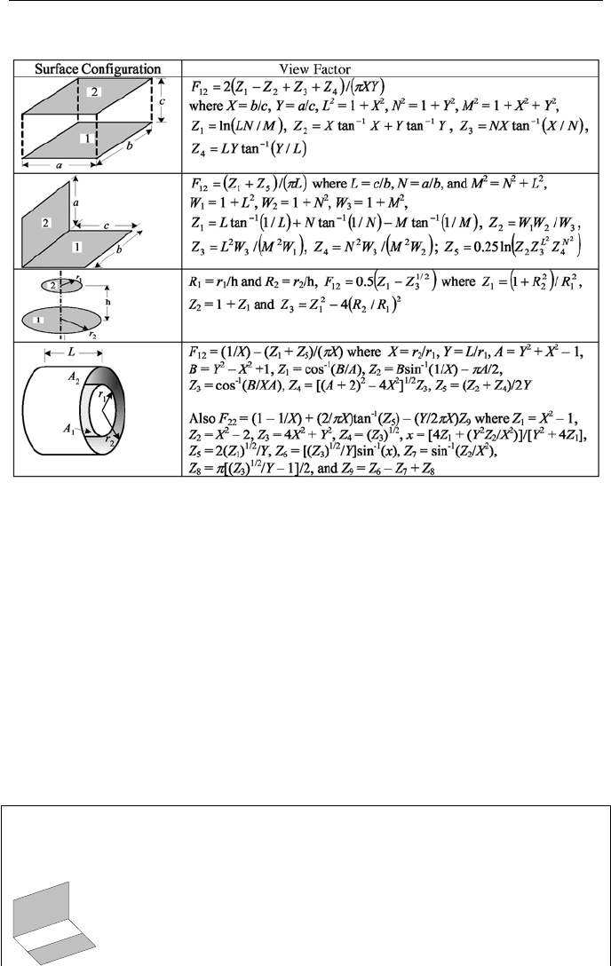
Table IVd.5.1. View factor for flat plates (Rohsenow 73)
5.2. View Factor Relations
Earlier we demonstrated that F
ij
A
i
= F
ji
A
j
. The reciprocity relation is useful in ob-
taining one view factor from the other known view factor. There are other useful
relations for the view factor. For example if we use a well insulated cube as an
enclosure, the view factor for a given side of this cube adds up to unity. This is
because each side of the cube has only five other sides of the cube for the ex-
change of radiant energy. Hence, the summation of all the fractions of the radiant
energy left the side of the cube adds up to unity. In general, for any enclosure we
can write
Σ
j
F
ij
= 1. We can also obtain view factor for non-standard orientations
from view factor for standard geometry and orientations.
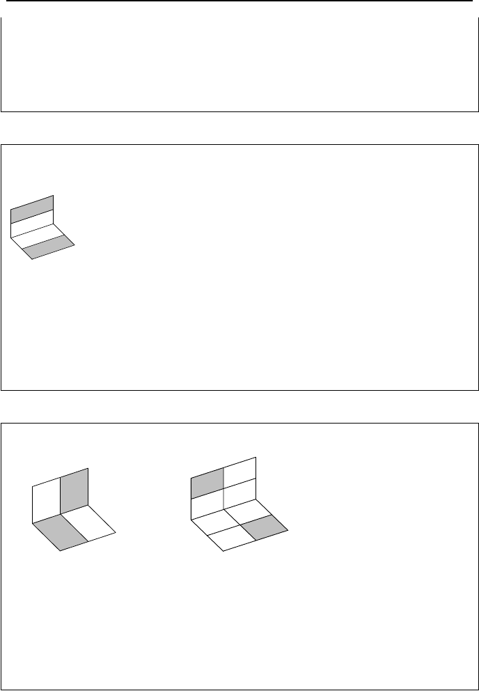
Example IVd.5.3. Find F
13
and F
31
for the arrangement below. All dimensions are
known.
1
2
3
584 IVd. Heat Transfer: Thermal Radiation
Solution: We reduce the view factor relations to obtain the intended view factor
from standard orientations:
A
1
F
1,23
= A
1
(F
12
+ F
13
). Hence, F
13
= F
1,23
– F
12
. To find F
31
we use the reciproc-
ity relation A
1
F
13
= A
3
F
31
.
F
31
= A
1
F
13
/A
3
= A
1
(F
1,23
– F
12
)/A
3
.
Example IVd.5.4. Find F
14
for the arrangement below. All dimensions are
known.
1
2
3
4
Solution: We reduce the view factor relations to obtain the intended view factor
from standard orientations: A
12
F
12,34
= A
1
F
1,34
+ A
2
F
2,34
. This can be further ex-
panded to:
A
12
F
12,34
= A
1
F
1,34
+ A
2
F
2,34
= A
1
(F
13
+ F
14
) + A
2
F
2,34
.
We still need to find F
13
. From the reciprocity relation we know that
A
1
F
13
= A
3
(F
3,21
– F
32
). Substituting, we get
F
14
= (A
12
F
12,34
+A
3
F
32
– A
2
F
2,34
– A
3
F
3.21
)/A
1
.
Example IVd.5.5. For the perpendicular rectangles in Figure (a), find F
14
.
1
4
2
3
1
4
2
3
(a) (b)
Solution: In can be shown that for the more general case of Figure (b):
A
1
F
14
= A
4
F
41
= A
2
F
23
= A
3
F
32
Returning to Figure (a), we note that:
A
12
F
12,34
= A
1
F
13
+ A
1
F
14
+ A
2
F
23
+ A
2
F
24
Substituting from the above rule (i.e., A
1
F
14
= A
2
F
23
), we find:
F
14
= (A
12
F
12,34
– A
1
F
13
– A
2
F
24
)/2A
1

5. Radiation Exchange Between Surfaces 585
Example IVd.5.6. Find F
12
and F
21
for a right circular cylinder of diameter D and
height H.
A
2
A
3
A
1
Solution: Using the summation rule for an enclosure, F
11
+ F
12
+ F
13
= 1.
Since F
11
= 0 and F
13
is known, we find F
12
= 1 – F
13
.
Finally, from the reciprocity relation, F
21
= A
1
F
12
/A
2
= A
1
(1 – F
13
)/A
3
5.3. Radiation Exchange Between Black Surfaces
Exchange of radiation between blackbodies is straightforward since a blackbody is
a perfect emitter and absorber. Consider for example black surface i exchanging
radiation with black surface j. The total rate of energy from surface i intercepted
by surface j is A
i
F
ij
J
i
. Similarly, the total rate of energy from surface j intercepted
by surface i is A
j
F
ji
J
j
. Since for black surfaces J ≡ E
b
, the net rate of radiant en-
ergy between blackbodies i and j is given by:
44
()
ij i ij i j
QAFTT
σ
=−
IVd.5.4
Example IVd.5.7. The cylinder in Example IVd.5.6 represents a furnace. Sur-
face A
1
is open to surroundings at 30 C while A
2
and A
3
are maintained at 500 C
and 700 C, respectively. Find the power required to maintain furnace at these
temperatures. There is no other heat loss from the furnace. D = 2 m, h = 1 m.
Solution: We treat surfaces A
2
and A
3
as black surfaces and find heat loss due to
radiation by assuming A
1
is a fictitious surface. Hence, A
2
and A
3
loose heat to A
1
,
which in turn looses heat to surroundings. Total heat loss is
=+=
3121
QQQ
)()(
4
1
4
3313
4
1
4
2212
TTFATTFA −+−
σσ
A
1
= A
3
=
π
D
2
/4 =
π
. We also find A
2
=
π
Dh = 2
π
From Figure IVd.5.2(c) or Table IVd.5.1: F
13
= F
31
= 0.382
From Example IVd.5.6: F
12
= 1 – F
13
= 0.618. Also F
21
= A
1
F
12
/A
2
= 0.309
=Q
(5.67E-8) × [2
π
× 0.309 × (773
4
– 303
4
) +
π
× 0.383 × (973
4
– 303
4
) = 99 kW
586 IVd. Heat Transfer: Thermal Radiation
5.4. Radiation Exchange Between Gray Surfaces
In the previous section, we noticed that the only complication in the analysis of
radiation exchange between black surfaces is the determination of the view factor.
Since other surfaces are not perfect emitters and also reflect a fraction of the inci-
dent energy, the analysis of radiation exchange becomes more complicated. To
simplify the analysis we make the following assumptions:
− all surfaces constitute an enclosure of nonparticipating medium
− all surfaces are diffuse, gray, and opaque
− temperature is uniform over the entire surface (i.e., isothermal)
− reflective and emissive properties are constant over the entire surface
− radiosity and irradiation are uniform over the entire surface
− heat conduction and heat convection mechanisms are absent
Consider the enclosure shown in the left side of Figure IVd.5.3. Details of surface
i of this enclosure are shown in the right side of Figure IVd.5.3. The unit area of
this surface receives irradiation G and emits radiosity J so that the net rate of en-
ergy loss from this surface is found as:
Q
= A(J – G) IVd.5.5
J
G
T, A,
ε
Q
.
Control Volume
Adiabatic Boundary
I
r
r
a
d
i
a
t
i
o
n
G
G
r
=
ρ
G
E
m
i
s
s
i
o
n
Re
f
l
e
c
t
i
o
n
E =
ε
E
b
Figure IVd.5.3. Radiation emission in an enclosure
We may eliminate G by using the definition of radiosity, being the summation of
emission and reflection:
J =
ε
E
b
+
ρ
G IVd.5.6
To eliminate
ρ
, we use the assumption that the surfaces are opaque;
ρ
= 1 –
α
.
This can be further simplified by noting that for gray surfaces,
α = ε
. Substituting
in Equation IVd.5.6., we get J =
ε
E
b
+ (1 −
ε
)G. We now solve this for G = (J –
ε
E
b
)/(1 –
ε
) and substitute for G in Equation IVd.5.5 and rearrange to get:
)/()1( A
JE
Q
b
εε
−
−
=
IVd.5.7
5. Radiation Exchange Between Surfaces 587
The advantage of arranging the result in the form of Equation IVd.5.7 is that it
lends itself to an electrical engineering analogy, the electric potential represented
by E
b
– J drives current Q
through the resistance (1 –
ε
)/(
ε
A). This is a very use-
ful approach, first suggested by Oppenheim, which allows problems involving
complex radiation exchange to be solved by network representation. Note that
Equation IVd.5.7 deals only with one surface. The rate of radiation exchange be-
tween two surfaces is given by Equation IVd.5.3. We can then summarize the
thermal resistance for radiation heat transfer as the surface and the space resis-
tances given as:
Surface resistance due to surface conditions: R
s
= (1 –
ε
)/(
ε
A)
Space resistance due to geometry and orientation: R
g
= 1/(A
i
F
ij
)
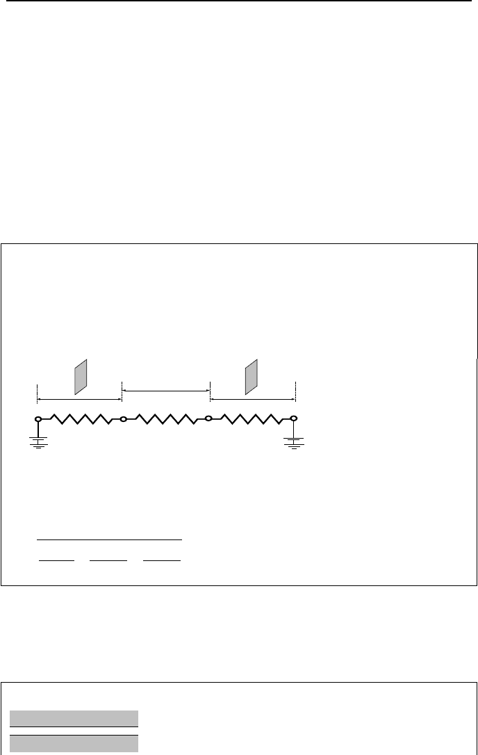
Example IVd.5.8. Two gray plates at T
1
and T
2
exchange radiation in a nonpar-
ticipating medium. Find Q
.
Solution: Here we deal with three radiation resistances namely, the surface resis-
tance of plate 1, the space resistance between plates 1 and 2, and the surface resis-
tance of plate 2, as shown in the figure:
J
1
J
2
E
b 2
E
b 1
(1-
ε
1
)/
ε
1
A
1
(1-
ε
2
)/
ε
2
A
2
1 /A
1
F
12
12
Space
Resistance
SurfaceResistance SurfaceResistance
Hence,
Σ
R = R
s1
+ R
g
+ R
s2
= [(1 –
ε
1
)/(
ε
1
A
1
) + 1/(A
1
F
12
) + (1 –
ε
2
)/(
ε
2
A
2
)] and
Q
= (E
b1
– E
b2
)/
Σ
R.
(
)
22
2
12111
1
4
2
4
1
1
1
1
AFAA
TT
Q
ε
ε
ε
ε
σ
−
++
−
−
=
IVd.5.8
We now apply Equation IVd.5.8 to four special cases including radiation ex-
change between parallel plates, long concentric cylinders, concentric spheres, and
a small surface encompassed by a large volume.
Example IVd.5.9. Find the net rate of heat transfer for two infinite parallel plates.
A
1
, T
1
,
ε
1
A
2
, T
2
,
ε
2

588 IVd. Heat Transfer: Thermal Radiation
Solution: For these plates, A
1
= A
2
= A and F
12
= 1. Therefore, from Equation
IVd.5.8, we find:
1/1/1
)(
21
4
2
4
1
12
−+
−
=
εε
σ
TTA
Q
Example IVd.5.10. Find the net rate of heat transfer for two infinite concentric
cylinders at radii r
1
and r
2
.
r
1
r
2
Solution: We use Figure IVd.5.2(d) for view factor between two concentric short
cylinders. When cylinders are long, F
12
= 1.0. Also substituting for A
1
= 2
π
r
1
L
and for A
2
= 2
π
r
2
L into Equation IVd.5.8, we find:
(
)
2
1
2
1
21
4
2
4
11
12
11
r
r
r
r
TTA
Q
−+
−
=
εε
σ
Example IVd.5.11. Find the net rate of heat transfer for two concentric spheres.
r
1
r
2
Solution: For these surfaces, A
1
/A
2
= (r
1
/r
2
)
2
and F
12
= 1 (note that F
22
≠ 0). Sub-
stituting these into Equation IVd.5.8, we obtain:
])/(/)/(/1/[)(
2
212
2
211
4
2
4
1112
rrrrTTAQ −+−=
εεσ
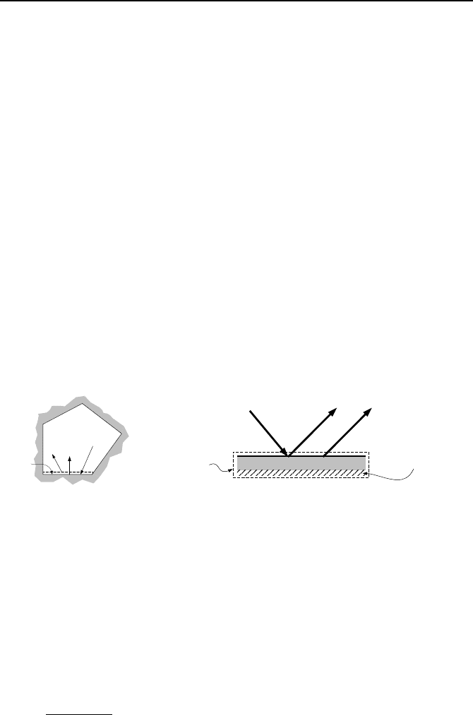
Example IVd.5.12. Find the net rate of heat transfer for a small convex surface
encompassed by a large cavity.
T
1
, A
1
,
ε
1
T
2
, A
2
,
ε
2
5. Radiation Exchange Between Surfaces 589
Solution: For these surfaces, A
1
/A
2
= 0 and F
12
= 1. Substituting these into Equa-
tion IVd.5.8, we obtain:
44
12 1 1 1 2
()QATT
σε
=−
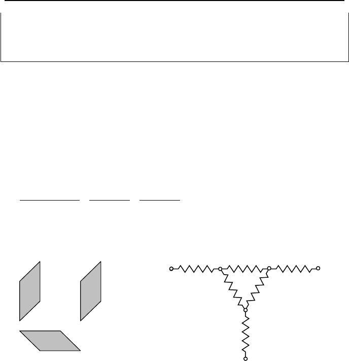
The method shown in Example IVd.5.7 can be extended to three surfaces ex-
changing radiation, as shown in Figure IVd.5.4. However, as the number of par-
ticipating surfaces increases, so is the number of equations. Since equations for
unknown radiosities are linear, an easy way to handle such cases is to set up a ma-
trix equation. Let’s consider surfaces 1 and 2 in an enclosure whose walls are rep-
resented by surface 3. At steady state conditions, the rate of heat transferred into
node J
1
is equal to the rate of heat transfer out of node J
1
(i.e., the net must be
zero):
0
)/(1)/(1)/()1(
131
13
121
12
111
11
=
−
+
−
+
−
−
FA
JJ
FA
JJ
A
JE
b
εε
1
2
3
A
1
T
1
ε
1
A
2
T
2
ε
2
A
3
T
3
ε
3
J
3
J
1
J
2
E
b2
E
b1
E
b3
(1-
ε
3
)/
ε
3
A
3
(1-
ε
1
)/
ε
1
A
1
(1-
ε
2
)/
ε
2
A
2
1
/
A
1
F
1
3
1
/
A
2
F
2
3
1/A
1
F
12
Figure IVd.5.4. Radiation exchange between three surfaces and the related radiation net-
work
We can write similar equations for nodes 2 and 3. If we generalize and con-
sider N gray and diffuse plates exchanging radiation, there will be N sets of linear
algebraic equations for N unknown radiosities. Thus, for N surfaces, the set of
equations may be arranged in a matrix equation of the form AX = B with the coef-
ficient matrix, the vector of unknowns and the vector of constants having the fol-
lowing elements:
590 IVd. Heat Transfer: Thermal Radiation
»
»
»
»
»
»
»
¼
º
«
«
«
«
«
«
«
¬
ª
−+−−−−−−
−−−+−−−−
−−−−−+−−
−−−−−−−+
¦
¦
¦
¦
NiNNNNNNNN
Ni
Ni
Ni
FFFF
FFFF
FFFF
FFFF
)1()1()1()1(
)1()1()1()1(
)1()1()1()1(
)1()1()1()1(
321
33333323313
22232222212
11131121111
εεεεε
εεεεε
εεεεε
εεεεε
"
#####
"
"
"
»
»
»
»
»
»
¼
º
«
«
«
«
«
«
¬
ª
N
J
J
J
J
#
3
2
1
=
»
»
»
»
»
»
¼
º
«
«
«
«
«
«
¬
ª
bNN
b
b
b
E
E
E
E
ε
ε
ε
ε
#
33
22
11
IVd.5.9
where index i in Equation IVd.5.9 ranges from 1 to N. Upon obtaining J
1
through
J
N
from Equation IVd.5.9, we then find the corresponding rates of heat transfer for
each surface from Equation IVd.5.7. Since the surfaces do not “see” themselves
(i.e., F
ii
= 0) then the diagonal terms become unity.
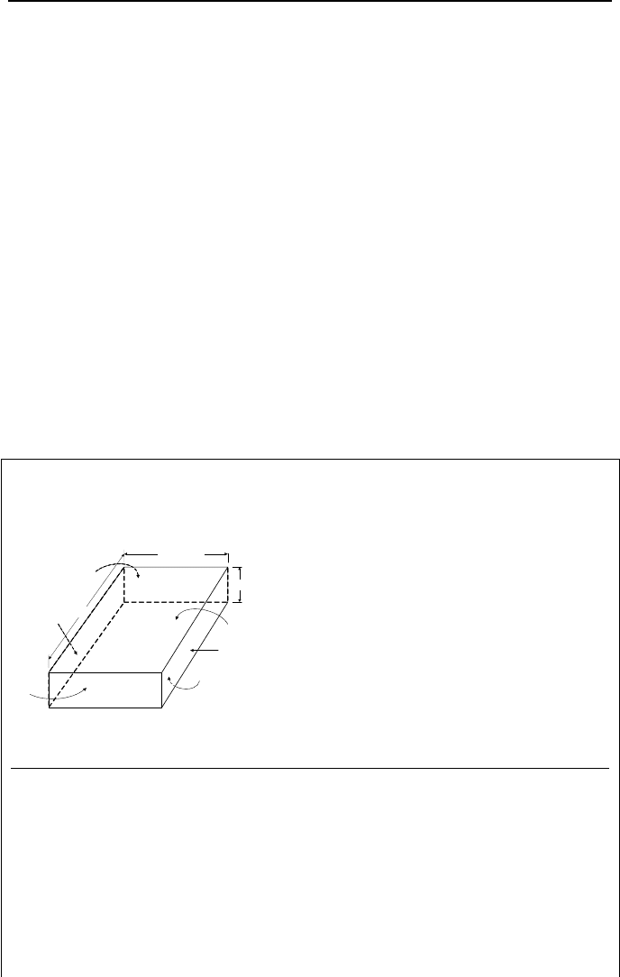
Example IVd.5.13. The gray and diffuse surfaces of a rectangular parallelepiped
are exchanging radiation with each other and nothing else. Use the following data
to find the related radiosities and the rate of heat transfer to or from each surface.
1 m
0.5 m
0.25 m
A
1
A
5
A
6
A
2
A
4
A
3
Surface No. T (K)
ε
A (m
2
) F: 1 2 3 4 5 6
1 500 0.3 0.500 F
1j
0.000 0.509 0.167 0.167 0.079 0.079
2 600 0.4 0.500 F
2j
0.509 0.000 0.167 0.167 0.079 0.079
3 550 0.8 0.250 F
3j
0.334 0.334 0.000 0.165 0.084 0.084
4 700 0.8 0.250 F
4j
0.334 0.334 0.165 0.000 0.084 0.084
5 650 0.6 0.125 F
5j
0.315 0.315 0.167 0.167 0.000 0.036
6 750 0.7 0.125 F
6j
0.315 0.315 0.167 0.167 0.036 0.000
Solution: The top and bottom surfaces are A
1
and A
2
, the left and right sides are
A
3
and A
4
, and the back and front surfaces are A
5
and A
6
. The above view factors
are found from Figures IVd.5.2(a) and IVd.5.2(b):

5. Radiation Exchange Between Surfaces 591
Parallel surfaces:
For A
1
– A
2
, X = 0.50, Y = 1.00, L = 0.25, and F
12
= F
21
= 0.509
For A
3
– A
4
, X = 0.25, Y = 1.00, L = 0.50, and F
34
= F
43
= 0.165
For A
5
– A
6
, X = 0.50, Y = 0.25, L = 1.00, and F
56
= F
65
= 0.036
Perpendicular surfaces:
For surfaces A
1
– A
3
, A
1
– A
4
, A
2
– A
3
, and A
2
– A
4
:
X = 1.00, Y = 0.50, Z = 0.25 resulting in:
F
13
= F
23
= F
14
= F
24
= 0.167 and F
31
= F
32
= F
41
= F
42
= (0.5/0.25) × 0.167 =
0.334
For surfaces A
1
– A
5
, A
1
– A
6
, A
2
– A
5
, and A
2
– A
6
:
X = 0.50, Y = 1.00, Z = 0.25 resulting in:
F
15
= F
16
= F
25
= F
26
§ 0.079 and F
51
=F
61
= F
52
= F
62
= (1.0/0.25) × 0.079 = 0.315
For surface A
3
– A
5
, A
3
– A
6
, A
4
– A
5
, and A
4
– A
6
:
X = 0.25, Y = 1.00, Z = 0.50 resulting in:
F
35
= F
36
= F
45
= F
46
= 0.084 and F
53
= F
63
= F
54
= F
64
= (1.0/0.50) × 0.084 =
0.167
The emissive powers are found from Equation IVd.2.1. For example, E
b1
=
5.67E–8 × 500
4
W/m
2
. If we now substitute values in Equation IVd.5.9, we find:
»
»
»
»
»
»
»
»
¼
º
«
«
«
«
«
«
«
«
¬
ª
−−−−−
−−−−−
−−−−−
−−−−−
−−−−−
−−−−−
00.101.005.005.009.009.0
01.000.107.007.013.013.0
02.002.000.103.007.007.0
02.002.003
.000.107.007.0
05.005.010.010.000.131.0
06.006.012.012.036.00.1
1
2
3
4
5
6
J
J
J
J
J
J
ªº
«»
«»
«»
«»
«»
«»
«»
«»
¬¼
=
»
»
»
»
»
»
»
»
¼
º
«
«
«
«
«
«
«
«
¬
ª
16.12558
78.6072
94.10890
72.4150
33.2939
12.1063
Upon solving this set, we find; J
1
= 7536.7 W/m
2
, J
2
= 8265.2 W/m
2
, J
3
= 6032.9
W/m
2
, J
4
= 12,556.5 W/m
2
, J
5
= 9522.8 W/m
2
, and J
6
= 15,085.6 W/m
2
. The cor-
responding rates of heat transfer for the surfaces are:
1
Q
=
()
()( )
4
(5.67E 8) 500 7536.3
10.3/0.30.5
−× −
=−
−×
855.6 W. Similarly, we find
2
Q
= –305.6
W,
3
Q
= –844.5 W,
4
Q
= –1057.2 W,
5
Q
= 112.2 W, and
6
Q
= 832.6 W.
Such problems involving radiation exchanges between isothermal surfaces can be
easily solved with the software included on the accompanying CD-ROM.
We use a similar method to solve problems in which instead of surface tem-
peratures, the surface heat flux is specified. An adiabatic surface is a special case
of the heat flux boundary conditions in which the heat flux is zero. Thus, if sur-
face i is adiabatic, then E
bi
≡ J
i
, which is equivalent with
ε
i
≈ 0.