Markowich P. Applied Partial Differential Equation: A Visual Approach
Подождите немного. Документ загружается.


7 Reaction-Diffusion Equations – Homogeneous and Heterogeneous Environments
115

7 Reaction-Diffusion Equations – Homogeneous and Heterogeneous Environments
116
Fig. 7.4. Fields in Guanxi Province, China
species of predators with concentration v (here u and v are scalar variables, note
the change of notation!), their interaction dynamics is modeled by:
u
t
= d
1
Δu + au − buv − fu
2
v
t
= d
2
Δv − dv + cuv − ev
2
,
where a, b, f , d, c, e, d
1
and d
2
are positive constants or parameter functions.
These reaction parameters can easily be interpreted. In the absence of predators
and without diffusion, the prey species satisfies a logistic equation, predict-
ing saturation at the value
a
f
, occuring with exponential speed at the rate a.
Moreover, in the absence of prey and without diffusion, the predators die
out exponentially, with exponential rate d. We remark that the parameters
f and e account for the strength of intra-species friction among prey and
predators resp. This friction, caused for example by competition for nutri-
ents, stabilizes the prey population even without predators. If both species
are present initially, then their respective rates of change are supposed to
be influenced by the number of their encounters, typically ending badly for
the prey, i.e. b>0, and good for the predator, i.e. c>0. Note that due to
the quadratic nature of the Lotka–Volterra system, only two-body interactions
prey-prey, predator-predator and predator-prey are taken into account by this
model.

7 Reaction-Diffusion Equations – Homogeneous and Heterogeneous Environments
117
The coefficients d
1
and d
2
determine the strength of diffusion of prey and
predators, resp. Obviously, the environment dependence can be accounted for
by making the coefficients x-dependent in an appropriate way.
The mathematicalliterature onreaction-diffusionequationsisvast.Asastan-
dard text we reference the textbook [9].
Typical mathematical questions in the theory of reaction-diffusion equations
deal with existence of solutions, global boundedness of solutions by means
of maximum and invariant region methods, large-time asymptotics, travelling
waves and geometry and topology of attracting sets, singular limits etc.
The maybe most basic mathematical question refers to the stability properties
of the reaction-diffusion system under consideration. For this, assume that, for
simplicity’s sake, D is independent of u and t, F independent of t and that
u
0
= u
0
(x) is a stationary state of the reaction-diffusion system, i.e.
0
= div (D(x)gradu
0
)+F(x, u
0
).
An important question concerns the behaviour of solutions of the nonlinear
system in comparism with the solutions of the linearized system, when the
linearization is performed at the stationary state u
0
, in direction of a function v:
v
t
= div (D(x)gradv)+D
u
F(x, u
0
)v .
Clearly, this is still a difficult problem in full generality (and also for many
particularly interesting cases). Thus, it seems intruiging to neglect diffusion
and to analyse the linear ODE system instead
w
t
= D
u
F(x, u
0
)w .
At least in the homogeneous case, where D, F and consequently u
0
are inde-
pendent of x, it suffices to calculate the eigenvalues of DF(u
0
)todecideabout
linearized, diffusionless stability. If all eigenvalues have negative real parts, then
only exponentially decaying modes of w exist, eigenvalues with positive real
parts generate exponential instabilities and more information is required if
eigenvalues with zero real part occur. In the first two cases the linearized be-
haviour carries over to the diffusionless nonlinear ODE system locally around
stationary points.
For example, take the predator-prey model formulated above. Then, neglect-
ing diffusion, a simple calculation shows the existence of two stationary states,
namely (0, 0) corresponding to extinction of both species and a state (u
0
, v
0
)with
u
0
=
ae + db
ef + bc
v
0
=
ac − df
ef + bc
.
Note that the predator-equilibrium value becomes negative unless ac − df > 0.

7 Reaction-Diffusion Equations – Homogeneous and Heterogeneous Environments
118
Fig. 7.5. Fields in Chiapas, Mexico
A simple calculation shows that the extinction state is the intersection of a
1-dimensional stable manifold corresponding to the predator species and an
unstable one corresponding to the prey species. The other stationary state is
stable (in the linearized sense when diffusion is neglected and when ac −df > 0).
A very interesting phenomenon happens when diffusion is taken into account
in the stability analysis. Although, intuitively speaking, diffusion stabilizes par-
ticle flow, there are cases of reaction-diffusion vector systems (d>1!) with
stationary points, which are exponentially stable in the diffusionless case AND
feature unstable modes if appropriate diffusion is taken into account. This so
called Turing instability (see [11]) is generated by sufficiently different diffu-
sivities for the different components of the vector u.Anexampleisgivenin
Chapter 4, in the context of biological pattern formation.
For analytical results on diffusive predator-prey models in heterogeneous
environments we refer to [3].
While modeling and analysis of reaction-diffusion systems in spatially un-
structured environments(i.e. the nonlinearity ofF and the diffusion matrix D are

7 Reaction-Diffusion Equations – Homogeneous and Heterogeneous Environments
119
independent of the position variable x) is by now a classical subject, the study
oftheinteractionofthespatialstructurewithreactionanddiffusionhasonly
started recently, particularly in biological/environmental/population dynamics
models. In this respect we cite [10]:
In the last two decades, it has become increasingly clear that the spatial
dimension and, in particular, the interplay between environmental het-
erogeneity and individual movement, is an extremely important aspect
of ecological dynamics.
In many cases when persistence of species or invasion of species into environ-
ments are analyzed, the standardassumption ofhomogeneity oftheenvironment
is obsolete and position dependent nonlinear reaction terms and diffusion ma-
trices have to be considered. Local environmental properties very often influence
individual survival and macroscopic persistence of species. For mathematical
results on reaction-diffusion equations in periodic media we refer to the re-

7 Reaction-Diffusion Equations – Homogeneous and Heterogeneous Environments
120
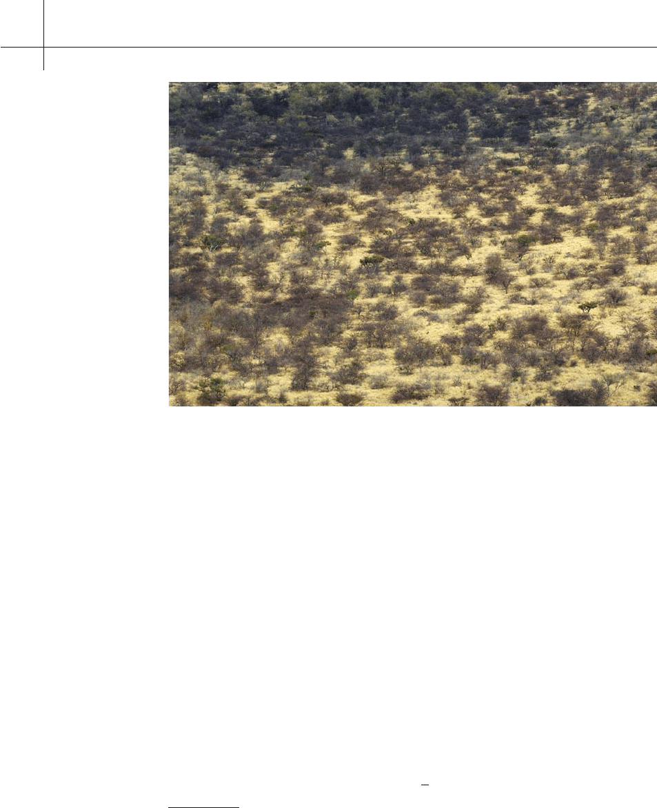
Fig. 7.6. Namibian savanna
cent papers of Henri Berestycki (and coworkers), which (among others) can be
downloaded from his webpage
6
.
Also, we point out the work of S.A. Levin
7
, in particular the review paper [6].
As an important and mathematically interesting example for the interaction
of heterogeneity and reaction-diffusion we mention homogenisation problems.
Consider a periodically fragmented environment, with a periodicity scale which
is small compared to the total characteristic dimension of the environment and
denote by the small positive parameter
ε the dimensionless ratio of these two
length scales, i.e. the microscopic-macroscopic ratio.
Then it is reasonable to assume that the diffusion matrix and the reaction
nonlinearity F are periodic in the position variable, with periodicity of the
order
ε. In precise terms, let
D
= D(y), F = F(y, u),
where D and F are periodic with respect to an n-dimensional lattice L (i.e. the
set of n-vectors with integer components) in y, define the fast scale
y
=
x
ε
6
http://www.ehess.fr/centres/cams/person/berestycki/
7
http://www.eeb.princeton.edu/∼slevin/

7 Reaction-Diffusion Equations – Homogeneous and Heterogeneous Environments
121
and consider the reaction-diffusion system
u
t
= div
D
x
ε
grad u
+ F
x
ε
, u
either on the whole space
R
n
or on a bounded domain with appropriate boundary
conditions.Forthesake of simplicity, we neglectedslowscaleeffects in D andin F.
The main questionis whether slow scale‘averaged’ dynamics can be extracted
from the fast scale problem without actually resolving the fast scale features. In
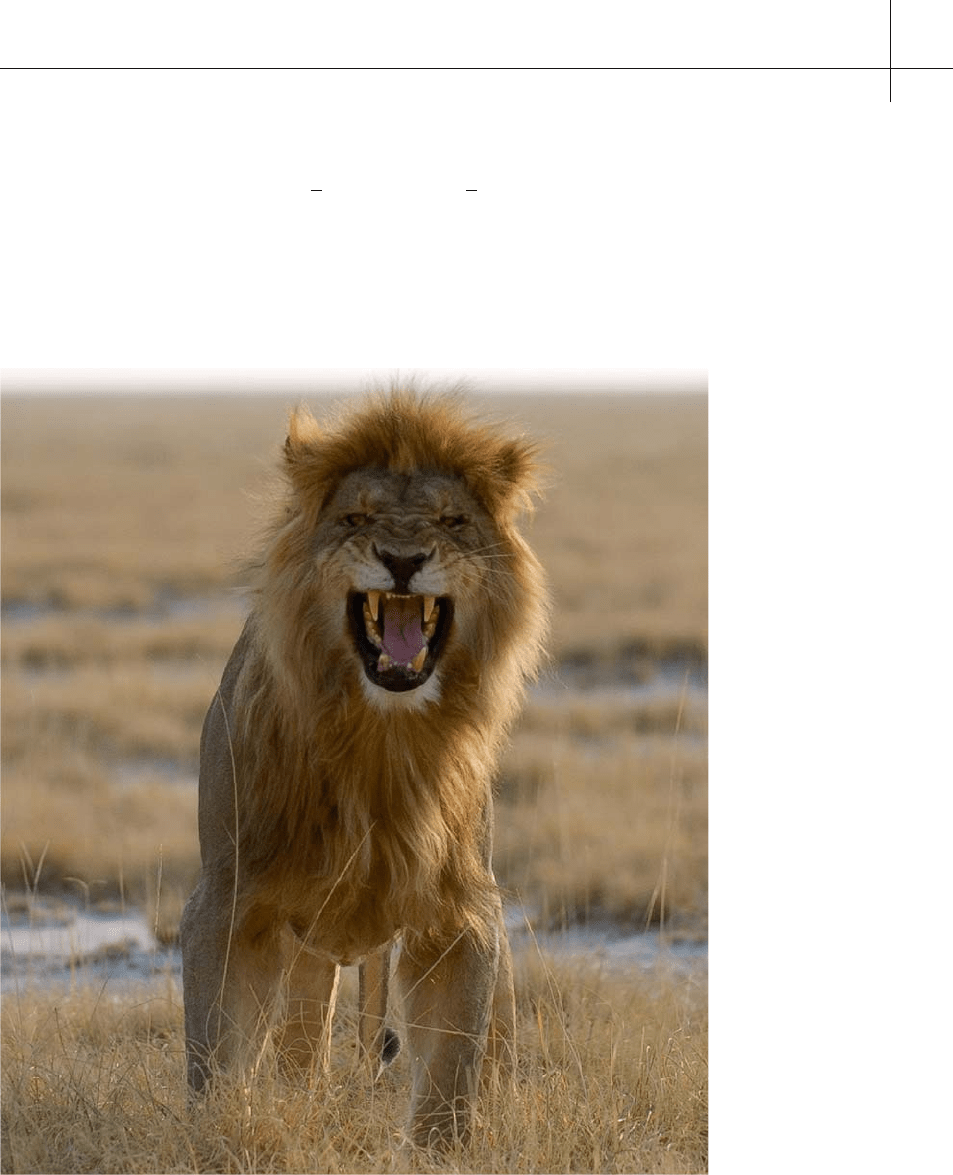
Fig. 7.7. Male lion

7 Reaction-Diffusion Equations – Homogeneous and Heterogeneous Environments
122
Fig. 7.8. Eagle
other words, does the solution u convergetoalimitasε converges to zero? If
yes, how can we characterize this limit?
For ‘good’ nonlinearities we expext a homogenized reaction-diffusion equa-
tion to hold for the limit u
0
,oftheform:
u
0
t
= div (D
0
grad u
0
)+F
0
(u
0
).
Here the ‘homogenized’ (constant coefficient) diffusion matrix D
0
is obtained
in analogy to the linear case by solving a cell problem (see [7], [2]) and F
0
is
obtained by computing the average of F(., u)overalatticecellC:
F
0
(u) =
1
vol C
C
F(y, u)dy.

7 Reaction-Diffusion Equations – Homogeneous and Heterogeneous Environments
123
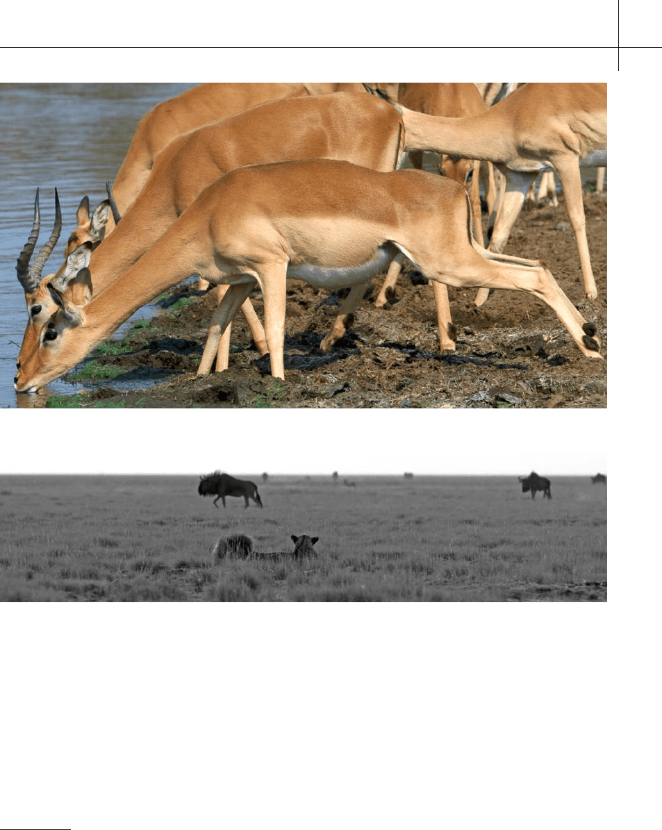
Fig. 7.9. Impala
Fig. 7.10. Predator and Prey
The theory becomes more involved, when slow scale dependence of D and/or F
is considered, too. Then double scale convergence techniques have to be applied.
Comments on the Images 7.1–7.5 The Images 7.1–7.3 show three dimensionally
terraced rice paddies
8
in the Chinese province Guanxi, close to the city of Guilin.
Clearly,theseareexcellentexamplesforheterogeneousbiologicalenvironments,
where heterogeneity is introduced through the topography of the hillside on
which the paddy is located and through the walls separating the paddies, which
inhibitthe global spreadof certain (invading or intentionally introduced) species
8
http://en.wikipedia.org/wiki/Paddy_field

7 Reaction-Diffusion Equations – Homogeneous and Heterogeneous Environments
124
or at least change their invasion patterns. Also we remark that the paddies are
connected by irrigation, which has to be included as a convection term into
the reaction diffusion system modeling biological populations in a terraced rice
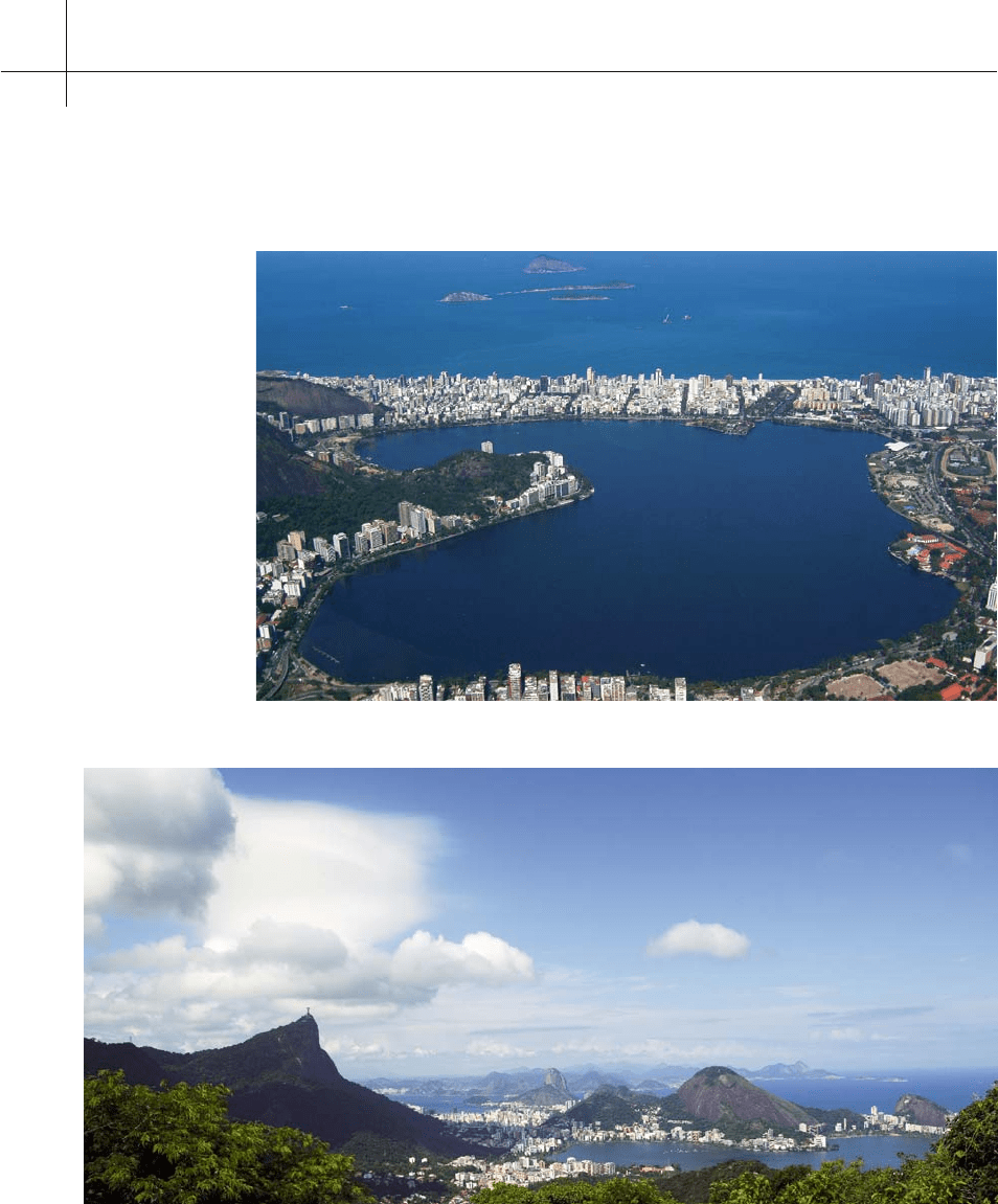
Fig. 7.11. Lagoa Rodrigo de Freitas, from Corcovado. Rio de Janeiro, Brazil
Fig. 7.12. Lagoa Rodrigo de Freitas ( foreground) and Guanabara bay, Rio de Janeiro, Brazil
