Lin S.D. Water and Wastewater Calculations Manual

Подождите немного. Документ загружается.

and from Thomas (1948)

(1.81)

then

(1.82)

Substitute t

in D

formula (Thomas, 1948):

(1.83)

(1.84)

Thomas (1948) provided this formula which allows us to approximate

: the maximum BOD load that may be discharged into a stream with-

out causing the DO concentration downstream to fall below a regulatory

standard (violation).

Example 1: The following conditions are observed at station A. The water

temperature is 24.3⬚C, with k

⫽ 0.06, k

⫽ 0.24, and k

⫽ 0.19. The stream

flow is 880 cfs. DO and L

for river water is 6.55 and 5.86 mg/L, respectively.

The state requirement for minimum DO is 5.0 mg/L. How much additional

BOD (Q ⫽ 110 cfs, DO ⫽ 2.22 mg/L) can be discharged into the stream and

still maintain 5.0 mg/L DO at the flow stated?

solution:

Step 1. Calculate input data with total flow Q ⫽ 880 ⫹ 110 ⫽ 990 cfs; at

T ⫽ 24.3⬚C

Saturated DO from Table 1.2

After mixing

6.55 3 880 1 2.22 3 110

990

5 6.07 smg/Ld

5 8.29 smg/Ld

log L

5 log D

1 c1 1

2 k

a1 2

0.418

log a

5 D

bc1 1

2 k

a1 2

0.418

sf 2 1d

logef c1 2 sf 2 1d

2 k

log

c1 2

2 k

Streams and Rivers 65

Deficit at station A

Deficit at critical point

Rates

Step 2. Assume various values of L

and calculate resulting D

Let L

⫽ 10 mg/L

Similarly, we can develop a table

Therefore, maximum L

a, max

⫽ 6.40 mg/L

, mg/L T

, days D

, mg/L

10.00 1.32 4.45

9.00 1.25 4.13

8.00 1.17 3.80

7.00 1.06 3.48

6.40 0.98 3.29

6.00 0.92 3.17

5 4.45 mg/L

5 0.792s10 3 0.561d

0.19

0.24

s10 3 10

20.1931.32

3 10

5 10.53 log s1.5 2 0.1665d 5 1.32 days

sf 2 1d

log ef c1 2 sf 2 1d

0.19s0.5d

log e1.5 c1 2 s0.5d

2.22

5 10.53 log a1.5 2

1.655

5 k

5 0.19 sper dayd

f 5

0.24

0.16

5 1.5

f 2 1 5 0.5

5 DO

2 DO

min

5 8.29 mg/L 2 5.00 mg/L 5 3.29 smg/Ld

5 DO

2 DO

5 8.29 mg/L 2 6.07 mg/L 5 2.22 smg/Ld

66 Chapter 1

Step 3. Determine effluent BOD load (Y

) that can be added

BOD that can be added ⫽ maximum load – existing load

This means that the first-stage BOD of the effluent should be less than

10.72 mg/L.

Example 2: Given: At the upper station A of the stream reach, under stan-

dard conditions with temperature of 20⬚C, BOD

⫽ 3800 lb/d, k

⫽ 0.14, k

⫽

0.25, k

⫽ 0.24, and k

⫽ k

. The stream temperature is 25.8⬚C with a veloc-

ity 0.22 mph. The flow in the reach (A S B) is 435 cfs (including effluent) with

a distance of 4.8 miles. DO

⫽ 6.78 mg/L, DO

min

⫽ 6.00 mg/L. Find how much

additional BOD can be added at station A and still maintain a satisfactory

DO level at station B?

Step 1. Calculate L

at T ⫽ 25.8⬚C

When t ⫽ 5 days, T ⫽ 20⬚C (using loading unit of lb/d):

Convert to T ⫽ 25.8⬚C:

Step 2. Change all constants to 25.8⬚C basis

At 25.8⬚C,

1sTd

5 k

1s20d

3 1.047

T220

1s25.8d

5 0.14 3 1.047

s25.8220d

5 0.18 sper dayd

2sTd

5 k

2s20d

3 s1.02d

T220

2s25.8d

5 0.25 3 s1.02d

25.8220

5 0.28 sper dayd

rs25.8d

5 0.24 3 1.047

s25.8220d

5 0.31 sper dayd

ds25.8d

5 0.31 sper dayd

asTd

5 L

as20d

[1 1 0.02sT 2 20d]

as25.8d

5 4750[1 1 0.02s25.8 2 20d]

5 5300slb/dd

3800 5 L

s1 2 10

20.1435

5 3800/0.80 5 4750slb/dd 5 L

as20d

y 5 L

s1 2 10

110Y

5 6.40 3 990 2 5.86 3 880

5 10.72 smg/Ld

Streams and Rivers 67

Step 3. Calculate allowable deficit at station B

At 25.8⬚C,

Step 4. Determine the time of travel (t) in the reach

Step 5. Compute allowable L

at 25.8⬚C using Eq. (1.69)

Here D

⫽ D

and D

⫽ D

Allowable load:

Step 6. Find load that can be added at station A

Step 7. Convert answer back to 5-day 20⬚C BOD

3680 5 L

as20d

[1 1 0.02s25.8 2 20d]

as20d

5 3297slb/dd

Added 5 allowable 2 existing

5 8980 lb/d 2 5300 lb/d

5 3680 slb/dd

lb/d 5 5.39 3 L

5 5.39s3.83 mg/Lds435 cfsd

5 8980

2.05 5

0.31L

0.28 2 0.31

s10

20.3130.9

2 10

20.2830.9

d 1 1.27 3 10

20.2830.9

2.05 5 s210.33dL

s0.526 2 0.560d 1 0.71

5 1.34 /0.35 5 3.83 smg/Ld

2 k

s10

2 10

d 1 D

3 10

t 5

distance

4.8 miles

0.22 mph 3 24 h/d

5 0.90 days

sat

5 8.05 mg/L

5 6.00 mg/L

5 8.05 mg/L 2 6.00 mg/L 5 2.05 mg/L

5 8.05 mg/L 2 6.78 mg/L 5 1.27 mg/L

68 Chapter 1

Example 3:

Given: The following data are obtained from upstream station A.

⫽ 0.14 @ 20⬚C BOD

load at station A ⫽ 3240 lb/d

⫽ 0.31 @ 20⬚C Stream water temperature ⫽ 26°C

⫽ 0.24 @ 20⬚C Flow Q ⫽ 188 cfs

⫽ k

Velocity V ⫽ 0.15 mph

⫽ 5.82 mg/L A–B distance ⫽ 1.26 miles

Allowable DO

min

⫽ 5.0 mg/L

Find: Determine the BOD load that can be discharged at downstream

station B.

solution:

Step 1. Compute DO deficits

At T ⫽ 26°C

⫽ 8.02 mg/L and D

at station A

⫽ DO

⫺ DO

⫽ 8.02 mg/L ⫺ 5.82 mg/L ⫽ 2.20 mg/L

Critical deficit at station B.

⫽ 8.02 ⫺ DO

min

⫽ 8.02 mg/L⫺ 5.0 mg/L ⫽ 3.02 mg/L

Step 2. Convert all constants to 26⬚C basis

At 26°C,

1s26d

5 k

1s20d

3 1.047

s26220d

5 0.14 3 1.047

5 0.18 sper dayd

2s26d

5 k

2s20d

3 s1.02d

26220

5 0.31 3 s1.02d

5 0.34 sper dayd

rs26d

5 0.24 3 1.047

5 0.32 sper dayd

2s26d

rs26d

0.34

0.32

5 1.0625

Streams and Rivers 69

Step 3. Calculate allowable BOD loading at station B at 26⬚C

From Eq. (1.84):

Allowable BOD loading at station B:

lb/d ⫽ 5.39 ⫻ L

(mg/L) ⭈ Q (cfs)

⫽ 5.39 ⫻ 5.52 ⫻ 188

⫽ 5594

Step 4. Compute ultimate BOD at station A at 26⬚C

Step 5. Calculate BOD at 26⬚C from station A oxidized in 1.26 miles

Time of travel,

5 1030 slb/dd

5 4536 3 0.227

5 4536s1 2 10

20.3230.35

5 L

s1 2 10

t 5

1.26 miles

0.15 mph 3 24 h/d

5 0.35 days

5 4536 slb/dd

5 4050s1 1 0.12d

aAs26d

5 L

[1 1 0.02 3 s26 2 20d]

5 4050 slb/d, at 208Cd

5 3240/s1 2 10

20.1435

5 BOD

loading/s1 2 10

log L

5 log D

1 c1 1

2 k

a1 2

0.418

d log a

log L

5 log 3.02 1 c1 1

0.32

0.34 2 0.32

a1 2

2.2

3.02

0.418

dlog 1.0625

5 0.480 1 [1 1 16 3 s0.272d

0.418

]0.0263

5 0.480 1 10.28 3 0.0263

5 0.750

5 5.52 smg/Ld

70 Chapter 1

Step 6. Calculate BOD remaining from station A at station B

Step 7. Additional BOD load that can be added in stream at station B (⫽x)

This is first-stage BOD at 26°C.

At 20°C,

For BOD

at 20⬚C (y

)

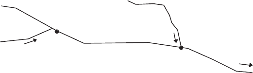
Example 4: Given: Stations A and B are selected in the main stream, just

below the confluences of tributaries. The flows are shown in the sketch below.

Assume there is no significant increased flow between stations A and B, and

the distance is 11.2 miles (18.0 km). The following information is derived

from the laboratory results and stream field survey:

⫽ 0.18 per day @ 20⬚C stream water temperature ⫽ 25⬚C

⫽ 0.36 per day @ 20⬚C DO above station A ⫽ 5.95 mg/L

⫽ 0.22 per day @ 20⬚C L

just above A ⫽ 8.870 lb/d @ 20⬚C

⫽ k

added at A ⫽ 678 lb/d @ 20⬚C

Velocity, V ⫽ 0.487 mph DO deficit in the tributary above

A ⫽ 256 lb/d

Find: Expected DO concentration just below station B.

118.9 MGD

11.2 miles

8.9 MGD

98.6 MGD

107.5 MGD

DO = 7.25 mg/L

11.4 MGD

5 x

s1 2 10

20.1435

5 1864 s1 2 10

20.7

5 1492 slb/dd

s26d

5 x

s20d

[1 1 0.02 3 s26 2 20d]

s20d

5 2088/1.12 lb/d 5 1864 slb/dd

s26d

5 allowable BOD 2 L

5 5594 lb/d 2 3506 lb/d

5 2088slb/dd

5 4536 lb/d 2 1030 lb/d 5 3506 slb/dd

Streams and Rivers 71

solution:

Step 1. Calculate total DO deficit just below station A at 25°C

DO deficit above station A D

⫽ 8.18 mg/L ⫺ 5.95 mg/L ⫽ 2.23 mg/L

lb/d of DO deficit above A ⫽ D

(mg/L) ⫻ Q (MGD) ⫻ 8.34 (lb/gal)

⫽ 2.23 ⫻ 98.6 ⫻ 8.34

⫽ 1834

DO deficit in tributary above A ⫽ 256 lb/d

Total DO deficit below A ⫽ 1834 lb/d ⫹ 256 lb/d ⫽ 2090 lb/d

Step 2. Compute ultimate BOD loading at A at 25⬚C

At station A at 20⬚C, L

⫽ 8870 ⫹ 678 ⫽ 9548 lb/d

At station A at 25⬚C, L

⫽ 9548[1 ⫹ 0.02(25 ⫺ 20)]

⫽ 10,503 lb/d

Step 3. Convert rate constants for 25⬚C

Step 4. Calculate DO deficit at station B from station A at 25⬚C

Time of travel t ⫽ 11.2/(0.487 ⫻ 24) ⫽ 0.958 days

Convert the DO deficit into concentration.

5 amount, lb/d/s8.34 lb/gal 3 flow, MGDd

5 2208/s8.34 3 107.5d

5 2.46 smg/Ld

2 k

s10

2 10

d 1 D

3 10

0.28 3 10,503

0.40 2 0.28

s10

20.2830.958

2 10

20.430.958

d 1 2090 3 10

20.430.958

5 24,507s0.5392 2 0.4138d 1 2090 3 0.4138

5 3073 2 865

5 2208slb/dd

1s25d

5 k

1s20d

3 1.047

s25220d

5 0.18 3 1.258

5 0.23 sper dayd

2s25d

5 k

2s20d

3 1.024

25220

5 0.36 3 1.126

5 0.40 sper dayd

rs25d

5 k

rs20d

3 1.047

25220

5 0.22 3 1.258

5 0.28 sper dayd 5 k

ds25d

72 Chapter 1

This is DO deficiency at station B from BOD loading at station A.

Step 5. Calculate tributary loading above station B

DO deficit ⫽ 8.18 mg/L ⫺ 7.25 mg/L ⫽ 0.93 mg/L

Amount of deficit ⫽ 0.93 ⫻ 8.34 ⫻ 11.4 ⫽ 88 (lb/d)

Step 6. Compute total DO deficit just below station B

Total deficit

Step 7. Determine DO concentration just below station B

DO ⫽ 8.18 mg/L ⫺ 2.23 mg/L ⫽ 5.95 (mg/L)

Example 5: A treated wastewater effluent from a community of 108,000 per-

sons is to be discharged into a river which is not receiving any other significant

wastewater discharge. Normally, domestic wastewater flow averages 80 gal

(300 L) per capita per day. The 7-day, 10-year low flow of the river is 78.64 cfs.

The highest temperature of the river water during the critical flow period is

26.0⬚C. The wastewater treatment plant is designed to produce an average car-

bonaceous 5-day BOD of 7.8 mg/L; an ammonia–nitrogen concentration of

2.3 mg/L, and DO for 2.0 mg/L. Average DO concentration in the river upstream

of the discharge is 6.80 mg/L. After the mixing of the effluent with the river

water, the carbonaceous deoxygenation rate coefficient (K

or K

) is estimated

at 0.25 per day (base e) at 20⬚C and the nitrogenous deoxygenation coefficient

or K

) is 0.66 per day at 20⬚C. The lag time (t

) is approximately 1.0 day.

The river cross section is fairly constant with mean width of 30 ft (10 m) and

mean depth of 4.5 ft (1.5 m). Compute DO deficits against time t.

solution:

Step 1. Determine total flow downstream Q and V

5 0.681 sft/sd

Velocity V 5 Q

/A 5 91.95 ft

/s s30 3 4.5d ft

5 91.95 cfs

Downstream flow Q

5 Q

1 Q

5 13.31 cfs 1 78.64 cfs

Upstream flow Q

5 78.64 cfs

5 13.31 cfs

5 8.64 3 10

gpd 3 1.54/10

cfs/gpd

Effluent flow Q

5 80 3 108,000 gpd

5 2208 lb/d 1 88 lb/d 5 2296 lb/d

5 2296/s8.34 3 118.9d

5 2.23 smg/Ld

Streams and Rivers 73

Step 2. Determine reaeration rate constant K

The value of K

can be determined by several methods as mentioned previ-

ously. From the available data, the method of O’Connor and Dobbins (1958),

Eq. (1.52) is used at 20⬚C:

Step 3. Correct temperature factors for coefficients

Zanoni (1967) proposed correction factors for nitrogenous K

in wastewater

effluent at different temperatures as follows:

(1.85)

and

(1.86)

For 26°C,

Step 4. Compute ultimate carbonaceous BOD (L

)

At 20°C,

At 26°C, using Eq. (1.28)

Step 5. Compute ultimate nitrogenous oxygen demand (L

)

Reduced nitrogen species (NH

⫹

, NO

, and NO

⫺

) can be oxidized aerobically

by nitrifying bacteria which can utilize carbon compounds but always

aCs26d

5 10.93 mg/Ls0.6 1 0.02 3 26d

5 12.24 smg/Ld

5 0.25 per day

BOD

5 7.8 mg/L

5 BOD

/s1 2 e

5 7.8 mg/L/s1 2 e

20.2535

5 10.93smg/Ld

Ns26d

5 0.66 per day 3 0.877

26222

5 0.39 sper dayd

NsTd

5 K

Ns20d

3 0.877

T222

for 22 to 308C

NsTd

5 K

Ns20d

3 1.097

T220

for 10 to 228C

2s26d

5 1.12 per day 3 1.024

26220

5 1.29 sper dayd

Cs26d

5 0.25 per day 3 1.047

5 0.33 sper dayd

5 13.0V

1/ 2

23/2

5 13.0s0.681d

1/2

s4.5d

23/2

5 1.12 sper dayd

74 Chapter 1