Kothari D.P., Nagrath I.J. Modern Power Systems Analysis
Подождите немного. Документ загружается.


"
l
Mod"rn Po*"r. Syrt"r An"lyri,
I
10
=
Bn
(100)2
Brr= 0'001
MW-r
Equation
(7.31)
for
plant
1 becomes
A.A2P;1+2^;B1P;1
+2^aBr2P62
=
^-76
(ii)
and for
plant
2
0.04Pc2+2ABrrP"r+Z)BuPcr=
)-20
(iii)
Substituting the
values
of
B-coefficients and )
-
25, we
get
Pct
=
128'57 MW
Pcz= 125 Mw
The transmission
power
loss
is
Pr
=
0.001
x
(128.57)'
=
16.53 MW
and the
load is
Po
=
Pct * Pcr- Pt-
=
128.57 + I25
-
16.53
-
237.04 MW
Consider
the system of Example
7 .4 with a load of
237 .04 MW at bus
2. Find
the optimum
load distribution
between the two
plants
for
(a)
when losses
are
included but
not coordinated,
and
(b)
when losses are
also coordinated.
Also
find
the savings in rupees
per
hour when losses are coordinated.
Solution Case a
If the transmission loss
is not coordinated,
the optimum
schedules
are obtained
by equating the incremental
fuel costs at
the two
plants.
Thus
0.02P-
+ 16=0.O4Pcz+20
The
power
delivered
to the load is
Pct * Pcz= 0.001P4r
+ 237.04
Solving
Bqs.
(i)
and
(ii)
for
P61 nncl P6.2,
we
get
Pcr
=
275.18 MW;
and Prr2
=
37.59 MW
Case
b This case
is already
solved in Example 7.4.
Optimum
plant
loadings
with
loss coordination
are
Pct= 128,57
MW; Pcz
=
125 MW
Loss
coordination causes the load on
plant
I to reduce
from 275.18 MW
to
128.57
MW.
Therefore, saving
at
plant
I due
to
loss
coordination is
(i)
(ii
)
Kgi:",+
16)dPc,
:
o.MPl,r
+r6Pctli),'r',
=
Rs 2,937.691hr
At
plant
2 the
load increases
from
37.59
MW
to 125
MW
coordination. The
saving at
plant
2 is
due
to
loss
=
-
Rs 2,032.431hr
The net saving
achieved
by coordinating
losses while
scheduling
the received
load
of
237.04 MW is
r'
2,937.69
-
2,032.43
=
Rs
g,OtS.Ztm,
Derivation
of Transmission
Loss
Forrnula
An accurate
method of
obtaining
a
general
formula
for
transmission
loss
has
been
given
by Kron
[4].
This, however,
is
quite
complicated.
The
aim
of
this
article is to
give
a simpler
derivation
by making
certain
assumptions.
Figure
7.9
(c)
depicts
the case
of two
generating
plants
connected
to an
arbitrary number of
loads through
a transmission
network.
One line
within
the
network is
designated as branch
p.
Im,agine
that the total load
current
1, is
supplied
by
plant
1 only,
as
in
Fig. 7.9a.
Let the current in line
p
& Irr.Define
\
(7.33)
(c)
Flg.
7.9 Schematic
diagram showing
two
plants
connected
through
a
power
network
to
a
number
of loads
Sirniinriv
with
nient
)
qinrnc
ctrnnirrino the fntel
lnqd
nnrant
t'Eic
? ok\ r'a ^a-
r^_-^,
vs^rvrrr
\r
r5.
,.rv), wv
v(ltl
define
I^n
Mrz=
i=
e.34)
tD
Mo1
wrd
Mp2 are
called curcent
distribution
factors.
The values
of current
distribution factors depend
upon
the impedances
of
the
lines
and
their
interconnection
and are independent
of the
current
Ip.

fW
Modern
power
Sygtem
Anatysis
t
When
both
generators
t and 2 are
supplying
current into
the network as
in
Fig.7.9(c),
applying the
principle
of superposition
the
current in the line
p
can
be
expressed
as
where
1ot and
Io2 are the
currents
supplied
by
plants
I and 2, respectively.
At
this stage let us
make
certain
simplifying
assumptions
outlined below:
(1)
All load currents
have
the same
phase
angle
with
respect to a common
refere{ce. To understand
the implication
of this assumption
consider the load
current at
the ith
bus. It can
be written
as
VDil I
(6t-
d)
=
lloil l1i
where
{.
is
the
phase
angle
of the bus voltage
and
/,
is the lagging
phase
angle
of the
load.
Since
{
and
divary
only through
a narrow
range at various
buses,
it is reasonable
to assume
that
0, is the
same for all
load
currents at all times.
(2)
Ratio
X/R is the
same
for all network
branches.
These two assumptions
lead
us
to
the conclusion
that Ip1
and I,
fFig.7
.9(a))
have the
same
phase
angle and
so have
Ioz and 1o
[Fig.
7.9(b)],
such that the
current
distribution factors
Mr, and Mr,
are real
rather than complex.
Let,
.
Ict
=
llcrl
lo, and lcz
=
1162l lo2
where
a, and
02 are
phase
angles
of 1",
and lor, respectiveiy
with respect
to
the
common reference.
From
Eq,
(7.35),
we
can write
llrl2
-
(Moll6l
cos
a1 +
Mpzllo2lcos
oz)2 a
(Mrll6lstn
o;
Mr2lls2lsn
oz)2 (7.36)
Expanding
the simplifying
the
above
equation,
we
get
ll,,l2
=
Mzrrllorlz +
tutf,zllczlz
+ 2MolMrzllctl
llGzlcos
(a1
-
oz)
ll.rl=
='?'
:II.J-
-&z-
sr
$lvtlcos/,
'
vL
Jllvrlcosf"
p
Substituting for llrl2 fromEq.
(7.37),
and
l1o,l and
llurl
from
Eq.
(7.38),'we
obtain
D2
D
r
Gr
rLu|rn,
"-
-
1v31"*fr)
p
*Wl,r,rMpzRp
lVllv2lcos
/,
cos
Q,
7
P
*
P3'
'
tvzP("o,
dritT
M32RP
(7
'3s)
Equation
(7
3e)
"T,o:
;:;::::;:,PczB,z
+
4,8,,
8..
-
'n-
WGoshfDmS,no
p
ffiDM"M"Ro
(7.40)
Bn
=
T.M',rR.
lV,l'
(cos
6)'
7
YL Y
The terms
Bs, Bp and 82,
are called
loss
cofficients
or B-cofficients.lf
voltages
are line
to
line
kV with resistances
in
ohms,
the
units
of B-coefficients
are in
MW-I. Further, with Po,
and Po,
expressed
in
MW,
P, will
also
be
in
MK
The\,bove results
can be extended
to the general
case
of
ft
plants
with
transrnishur loss expressed
as
kk
P,
=Df
PG^B^.PG.
m:l
n:l
where
cos
(a,,
-
on)
Brz
Now
(7.37)
(7.38)
where
Pot and Po, are
the three-phase
real
power
outputs
of
plants
I and 2
at
power
factors
of cos
(t,
and
cos
Q2,
and
yl
and
V2
are
the bus voltages at
the
plants.
ff Ro is
the resistance
of branch
p,
the
total transmission
loss is
given
by*
(7.41)
(7.42)
'The
general
expression for
the
power
system with
t
plants
is expressed as
P
F3'
T,*3,R,t.
.-r4r-lu|*ry
'r
-
1yf
1*r6f
L'
'nt"P
'
'
'
tVr,l2
1cosffi
Lu'
8
r,,,
=
lv-llv,lcosQ-
cosQ-
It can be recognized as
cos(a,
-
on)
lcosQ*cosQ,
Pcn
ilV,
Pc^
lV*
P'o4oo
*
zDpG^B^npGn
m,n:l
;!l
e,
=
lstrp(
Re
Pr=
ftrB,
*
...*
i?ffil
ruodern
power
system
nnatysis
I
The following assumptions
including
those mentioned
already are necessary,
if
B-coefficients
are
to be treated as
constants as total
load and load sharing
between
plants
vary. These assumptions
are:
1,
All load
currents maintain a constant
ratio to the total current.
2.
Voltage
magnitudes
at all
plants
remain
constant.
3. Ratio of
reactive to real
power,
i.e.
power
factor at each
plant remains
constant.
4.
Voltage
phase
angles at
plant
buses
remain fixed.
This is equivalent
to
assuming that the
plant
currents
maintain constant
phase
angle
with
respect to the
common reference, since source
power
factors
are assumed
constant as
per
assumption
3
above.
In spite of the number of
assumptions
made, it is fortunate
that treating
B-
coefficients
as constants,
yields
reasonably
accurate results, when
the
coeffi-
cients are calculated
for some
average operating
conditions.
Major system
changes require
recalculation of
the
coefficients.
Losses as a function
of
plant
outputs
can be expressed
by other
methods*,
but
the simplicity
of loss
equations is the chief
advantage
of the B-coefficients
method.
Accounting
for transmission
losses results
in considerable
operating
economy. Furthermore,
this consideration
is equally
important
in future system
planning
and, in
particular, with
regard
to the location
of
plants
and
building
of new transmission
lines:
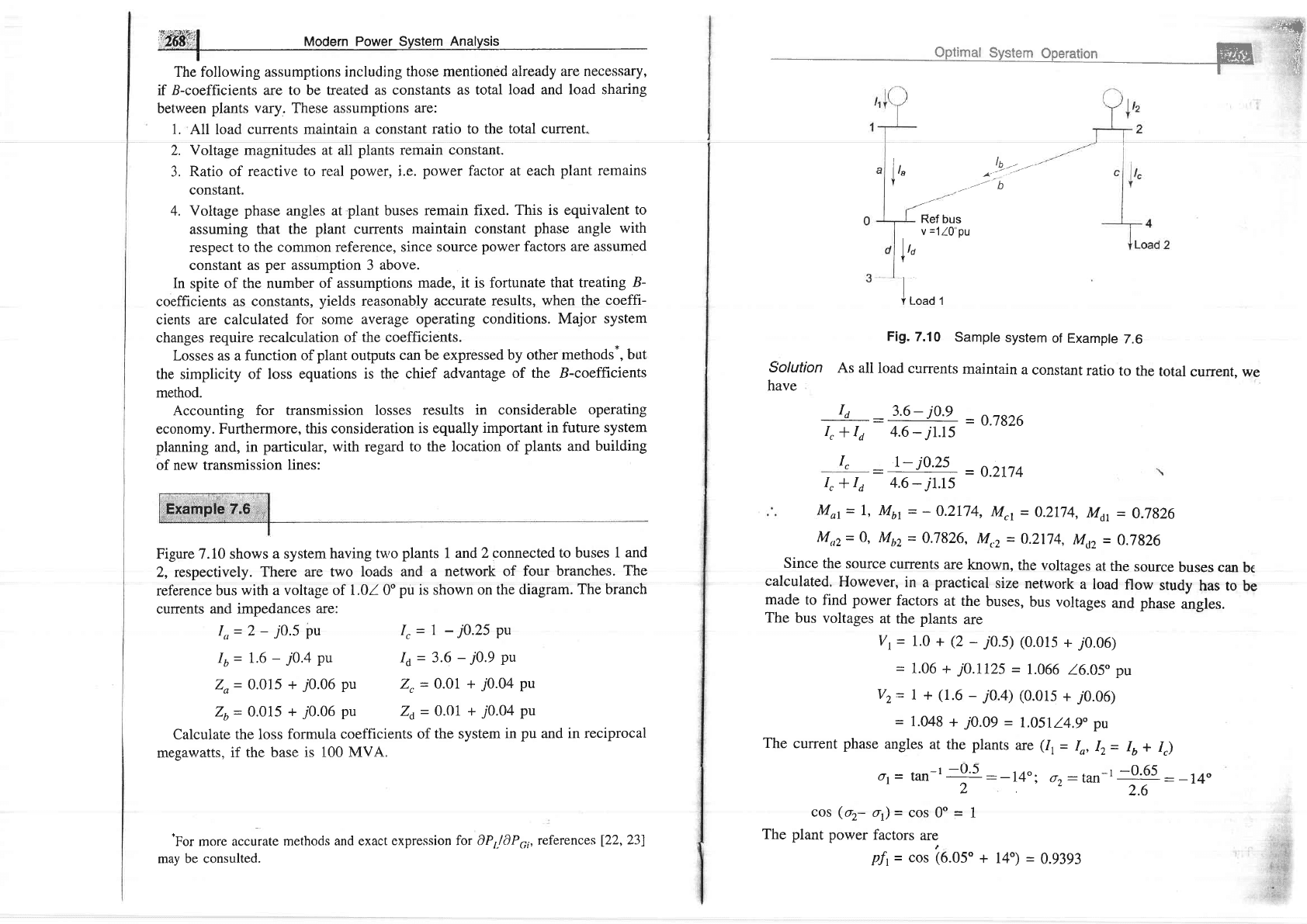
Figure 7.10
shows a system
having trrvo
plants
1
and 2 connected
to buses 1
and
2, respectively. There
are two
loads and a
network of four
branches.
The
reference
bus
with a voltage of l.0l0o
pu
is shown on
the diagram.
The
branch
cunents
and impedances
are:
Io=2
-
70.5 Pu
Iu= 1.6
-
j0.4
Pu
Zo
=
0.015
+
70.06
pu
Zo
=
0.015
+
70.06
pu
I,=7
-
j0.25Pu
Id
=
3.6
-
70.9 Pu
Z,
=
0.OI +
70.04
pu
Za
=
0.Ol
+
70.04
pu
Calculate
the loss
formula coefficients
of
the system
in
pu
and in reciprocal
mesawatfs if the hase is 100 MVA
^^^-D-
*For
more accurate
methods
and exact
expression for 0P,./0P6i,
references
122,231
may be consulted.
..-#
r !nrr!-na!
ffi i
-ii
lr"
Y
Ref bus
v
=1
10"
pu
l,o
Y
I ro"o r
Fig.
7.10
Sample
system
of
Example
7.6
Solution
As
all load
currents
maintain
a
constant
ratio
to the
total
current, we
have
rd
_
3.6_
jo.g
_
o.t8z6
I,
+
Id
4.6
-jl.l5
r-
i0.25
:
-
"----
-0.2174
4.6
-j1.1s
lb--
-
1''
----t''
b
I"
I,+ld
Mor=
L,
Mtr
-
-
0.2174,
Mrr
=
0.2774,
Mu
=
0.7826
M,,2= 0,
Mnz
=
0.7826,
Mrz
=
0.2174,
Mrtz
=
0,7826
Since
the source
currents
are
known,
the
voltages
at
the
source
buses can
be
calculated.
However,
in
a
practical
size
network
a load
flow
study
has to
be
made to
find
power
factors
at
the
buses,
bus voltages
and
phase
angles.
The
bus voltages
at
the
plants
are
Vr
=
1.0 +
(2
-
j0.5)
(0.015
+
70.06)
=
1.06 +
jO.I725 =
1.066
16.05"
pu
Vz=
7 +
(1.6
-
jO.4)
(0.015
+
70.06)
=
1.048
+
jO.O9 =
1.051
14.9" pu
The
current phase
angles
at the plants
are
(1,
=
Io,
12=
16r
Ir)
ot=
tan-t
+!.
:-
l4oi
o2:tan-r
-^O
9t
:
-
l4o
-22.6
cos
(or-
ot)
=
cos
0o
=
1
The plant
power
factors
are
pfi
=
cos
(6.05"
+ l4')
=
0.9393
ffiffi
Mociern
Power
Svstem
Ana[,sis
Pfz
=
cos
(4.9
+
14")
-
0.946
The
loss
coefficients
are
lBq.
Q.a\l
-
0.02224 pu
0.0 |
5
x
(0.7
82q2
+
0.0 1 x
(0.217
q2
+
0.01
x
(0.7
82q2
(1.051)2
x(0.946)2
=
0.01597
pu
D _
e0.2174)L0.7826X0.015) +
0.01x
(0.217a)2
+
0.01
x(0.7826)2
D
t2
=
rJ66 .
Lotl
x
0.9393 x
0.946
=
0.00406 pu
For
a base
of 100
MVA,
these
loss
coefficients
must
be
divided
by 100
to
obtain
their
values
in units
of reciprocal
megawatts,
i.e.
h
0.02224
Drr
=
LLL+
-
0.02224 x
lo2
Mw-l
100
8.t.,
=
0'01597
=
0.01597 x
1o-2
Mw-l
100
Br.t
=
0'0M06
=
0.00406
x
lo-z
Mw-l
100
7.6
OPTIMAL
LOAD
FLOW
SOLUTION
The
problem
of optimal
real
power
dispatch
has been
treated
in
the earlier
section
using
the
approximate
loss formula.
This
section presents
the
more
general
problem
clf real
attd reactive povrer
flow
so
as to
minirnize
the
instantaneous
operating
costs.
It is
a static
optimization
problem
with a
scalar
objective
function
(also
called
cost
function).
The
solution
technique given
here
was
first
given
by Dommel
and
Tinney
[34].
It
is
based
on
load
flow
solution
by the
NR method,
a first order
gradient
adjustment
algorithm
for
minimizing
the
objective
function
and
use of
penalty
functions
to account
for inequality
constraints
on clepenclent
variables.
The
problem
of unconstrained
optirnal
load flow
is
first tackJed.
Later the inequality
constraints
are
introduced,
first
on control
variables
and then
on dependent
variables.
Optimal
Power
Flow
without
Inequality
Constraints
The
objective
function
to
be
minimized
is
ihe
operating cost
Bzz
]=
tr4n
I
4 i
a.
slack
bus
4l
O
]
for
each
pe
bus
OPtimal
System
Operation
ffi
ffi$ffi
pl
c
=
f
ci(Pci)
e
-f
tUilvjily,,tcos(0,,
-
j:1
3
Q,
+
Ltvinvjlllzulsin
(0u
l
j:r
and
A
4
-
Llvllvjlly,,lcos(9,,
*
6i
-
4)=
0
for
each
pv
bus
j:7
It
is
to
be
notecl
that
at
the
ith
bus
Pt=
Pci-
Poi
Qi=
Qci-
Qu
where
Po,
and
ep;
are
load
demands
at
bus
i.
Equarions
(7.43),
(7.44)
and (7.45)
can
be
expressed
in
vector
form
[Eq.
(7.a3)l
I
'
f
(x,
y)
=
| _tn. \7qql
for
each
r0
bus
|
\
lEq. Q.a,
for
each
pV
bus
i
;
where
the
vector
of
dependent
variables
is
l-t
y,
tl
I
.=
lr,
jforeachrouusf
Ld,
for
each
pV
bus_J
and
the
vector
of
independent
variables
is
,1,,,j
t"each
PV
bus
fn fha
ql-^.ro
f^*,,.t^+:^- -r
qvvvv
rt-lrurulalLlull,
[fle
ODleQtlVe
tltnefinn mrrcf i_^1,-A^ d^^ _r
-
power.rrruDllllwlLlLlgLllESracKDuS
The
vector
of
independent
variabres
y
can
be partitioned
into
two
parts_a
vector
u of
control
variables
which
are
to
be
variea
to
achieve
optimum
value
of
the
objective
function
and
a vector
p
of
fixed
or
disturbange
or
unconhollable
(7.43)
(7.44)
(7.4s)
(7.46)
(7.47)
(7.48a)
(7.48b)
(7.7)
subject
to
the
load
flow
equations
[see
ffi@
Modern
Power
Svstem
Analvsis
puru-"t"rs.
Control
parameters*
may
be
voltage
magnitudes
on
PV
buses,
P6t
buses
with
controllable
power,
etc.
The
optimization
problem**
can
now
be
restated
as
min
C
(x'
u)
at
(7.4e)
subject
to equalitY
constraints
.f
(x,
u,
p)
=
0
(7'50)
To
solve
the
optimization
problem,
define
the
Lagrangian
function
as
L
(x,
u,
p)= C
(x,
u7+
Arf
(x,
u,
P)
(7'51)
where
) is
the
vector
of
Lagrange
multipliers
of
same
dimension
as
f
(x,
u,
p)
The
necessary
conditions
to minimize
the
unconstrained
Lagrangian
function
are
(see
Appendix
A
for
differentiation
of
matrix
functions).
af,
=
0c
*ly1'
)_o
0x
0x
L}x
J
0L
=
0c
*ly1'
)_o
0u
0u
Ldu-J
,
ar
u;
=
f
(x,
u,
P)
=
o
Equation
(7.54)
is
obviously
the
same
as
the
equality
(7.s2)
(7.s3)
(7.s4)
constraints.'
The
tS
^a
L
as
needed
in
Eqs.
(i.52) and
(7.53)
are
rather
expressions
for
;
0u
involved***.
It may
however
be observed
by
comparison
with
Eq.
(6.56a)
that
Y=
Jacobian
matrix
[same
as
employed
in
the
NR
method
of
load
flow
0x
solution;
the
expressions
for
the
elements
of
Jacobian
are
given
in Eqs.
(6.64)
and
(6.65)1.
Equations
(7.52),
0.53)
and
(7.54)
are
non-linear
algebraic
equations
and
can
only
be solved
iteratively.
A simple
yet
efficient
iteration
scheme,
that
can
by
employed,
is
the
steepest
descent
method
(also
called
gradient method).
-Slack
bus
voltage
and
regulating
transformer
tap
setting
may
be
employed
as
additional
control
variables.
Dopazo
et
all26ltuse
Qo,
as
control
variable
on
buses'
with
reactive
Power
control'
**rr
*L^ ..,.*^- .pal nnrrrcr lncc ic to he minimized- the obiective
function
is
lI
LrMJ
Dlvrrl
lvsr
rv
C
=
Pr(lVl,
6)
Since
in this
case
the
net
injected
real
powers
are fixed,
the minimization
of
the real
injected
power P,
at
the
slack
bus
is equivalent
to minimization
of
total
system
loss,
This
is
known
as
optimal
reactive
power
flow
problem'
***The
original
pup".
of Dommel
and
Tinney
t34l
may
be consulted
for
details'
feasible
solution
point
(a
set
of
values
of x
which
satisfies
Eq.
(7.5a)
for given
u and
p;
it indeed
is the load
flow
solution)
in
the direction
of steepest
desceht
(negative
gradient)
to a new
feasible
solution point
with
a lower
value
of
objeetlve funstion.
By repeating
the-.se
moves
in
*rc
dkestisn
+f the
negadve
gradient,
the minimum
will
finally be
reached.
The computational procedure
for the
gradient
method
with
relevant
details
is
given
below:
Step I
Make an initial
guess
for u,
the
control
variables.
Stey 2
- Jind
a feasible
load
flow solution
from
Eq.
(7.54)
by the
NR iterative
method. The
method
successively
improves
the
Solution
x as
follows.
*
(r
+r)
-
,(r) +
Ax
where
A-r is obtained
by
solving the
set of linear
equations
(6.56b)
reproduced
below:
rhe
end resurts
"^-,
J,;; $;
Iti.[l]'*u,,on
or
x and
the
racobian
matri,...
Step
3
Solve Eq.
(7.52)
for
(7.s5)
I
Step 4 Insert
) from Eq.
(7.55)
into
Eq.
(7.53),
and
compute
the
gradient
l#r,"',rl]4"
-
-
r
(*('),
y)
r, ^- -rr-l
\=-i
({\'l
ac
L\dxl J
0x
(7.s6)
It
may be noted
that for computing
the
gradient,
the Jacobian
J
-
+
is
already
0x
known from the load
flow solution
(step
2
above).
step 5 rf
v
-c
equals
zero
within
prescribed
tolerance,
the
minimum
has
been reached.
Otherwise,
Step
6 Find a new set
of control
variables
where
unew=
l.l.^6*
L,il
L,u
=
-
o"V-C,
Here A,u
is a
step in the
negative
direction
of the
gradient.
The
step
size
is
adjusted
by
the
positive
scalar
o..
Y.c,
=
oc
*l
9L1'
t
0u L0u )
(7.57\
(7.s8)
#*ff"
f
uooern Power
Svstem
Analvsis
Steps
1 through
5
are
straightforward
and
pose
no computational problems.
Step 6
is the critical
part
of the algorithm,
where the choice
of a is
very
important.
Too small
a value of
a
guarantees
the convergence
but
slows down
the
rate
of convergence;
too high
a value
causes
oscillations around
the
Inequality
Constraints
on
Control Variables
Though
in the
earlier
discussion,
the control
variables are
assumed to
be
unconstrai""o,
1.j":T.1",::tutt
are, in fact,
always
contrained,
(7.se)
e.g.
Pc,,
,nin
1
Po,
S
Pct,
**
These
inequality
constraints
on control variables
can be easily handled.
If the
correction
Au,inBq.
(7
,57) causes uito
exceed
one
of
the limits,
a, is set equal
to the
corresponding
limit, i.e.
to
the
constraint
limits,
when
these
limits
are
violated.
The penalty
function
method
is valid in
this
case,
because
these
constraints
are
seldom
rigid
limits
in
the strict
sense,
but
are in
fact,
soft
limits
(e.g.
lvl
<
1.0
on a
pebus
really
ry
v-should
not
exceed
1.0
too
much
and
lvl
=
1.01
may
still
be
The
penalty
method
calls
for
augmentation
of
the
objective
function
so that
the
new
objective
function
becomes
Ct=C(x,u)*
fUt
where
the
penalty
W, is introduced
for
each violated
inequality
constraint.
A
suitable penalty
function
is
defined
as
w,
=
{7i@i
-
xi,^o)2
i
whenever
xi
) xi,rnax
'
[
71G,-xi,^i)zi
wheneverxr(ry,min
Q'64)
where
Tiis
Treal
positive
number
which
controls
degree
of
penalty
and
is
called
the
penalty
factor.
Xmln
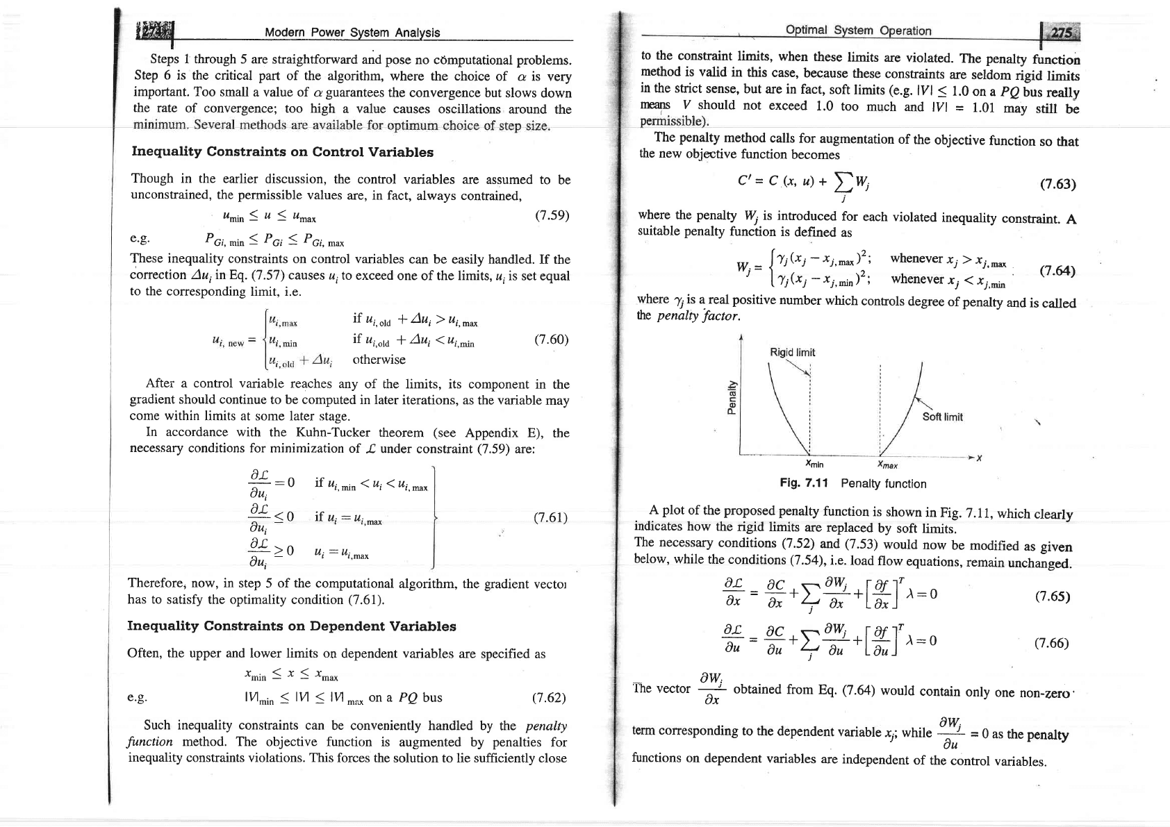
Fig.
7.11
Penalty
function
A
plot
of
the
proposed
penalty
function
is
shown
in
Fig.
7.11,
which
clearly
indicates
how
the rigid
limits
are replaced
by
soft
limits.
The
necessary
conditions
(7.52)
and
(7.53)
would
now
be
modified
as
given
below,
while
the conditions
(7.54),
i.e.
load
flow
equations,
remain
unchanged.
(7.6s)
(7.66)
(7.63)
if
u,,oro
*
Au,
)
ui,^^
7f
u,,oro
*
Au,
1ui,^in
otherwise
(7.60)
(7.6r)
After
a control variable
reaches
any
of the limits, its component
in
the
gradient
should
continue
to be
computed
in later
iterations, as
the
variable
may
come within
limits at
some later stage.
In
accordance with
the Kuhn-Tucker
theorem
(see
Appendix E),
the
necessary
conditions for
minimization of
I,
under
constraint
(7.59)
arc:
0L
:0
0u,
of
.o
ou,
-
or,o
0r,
-
Thereforer
now, in
step
5
of the
computational
algorithm, the
gradient
vector
has to
satisfy the optimality
condition
(7.61).
Inequality
Constraints on Dependent
Variables
Often, the upper and
lower limits on
dependent variables
are specified
as
rmir,SxSr*u^
e.g.
lUn,in
<
lVl
<
lYl
-.o
ofl
a
PQ
bus
(7.62)
Such inequality
constraints
can
be conveniently handled
by the
penalty
function
method. The
objective function
is augmented by
penalties
for
inequality
constraints violations. This
forces the
solution to lie sufficiently close
^trZ
UW:
'Ihe
vecto
obtained
from
Eq.
(7.64)
would
contain
only
one
non-zero.
0x
term
corresponding
to the
dependent
variable
x;;
while
#
=
0 as
the
penalty
functions
on
dependent
variables
are
independent
of
the
control
variables.
7f u,,*n
<ui
<ui,^^,
if u,
-
ui,^*
ui: ui.^u*
ax
_ac,\-awj
,f
afl',
T-
=
__l_
)
dx
ox
4ar*La"i)-o
l
ax
_AC,sdw;
,f
Af1',
-:-
=
--L
)
du
ou'+
a"*La"l'r:o
'
Modern
Power System
Analysis
By choosing
a higher
value
fot
1,,the
penalty
function
can be
made
steeper
so
that the
solution
lies
closer
to the
rigiA fimits;
the convergence,
however,
will
become
poorer. A
good
scheme
is to start
with
a
low
value of
7
j
and
to
increase
imization
process,
if the
solution
exceeds
a
certain
tolerance
limit.
This
section
has
shown
that
the
NR
method of
load
flow
can
be extended
to
yield
the
optimal
load flow
solution
that
is feasible
with
respect
to
all
relevant
inequality
constraints.
These
solutions
are often
required
for
system
planning
and
operation.
7.7 OPTIMAL
SCHEDULING
OF
HYDROTHERMAL
SYSTEM
The
previous sections
have
dealt
with the
problem
of
optimal
scheduling
of
a
Dower
system
with
thermal
plants only. Optimal
operating
policy in this
case
can
be completely
determined
at
any instant
without
reference
to
operation
at
other
times.
This,
indeed,
is
the static
optimization
problem.
Operation
of
a
system
having
both
hydro
and
thermal
plants
is,
however,
far
more
complex
as
hydro
plants have
negligible
operating
cost, but
are
required
to operate
under
constraints
of
water
available
for
hydro
generation
in
a
given period
of time.
The
problem
thus belongs
to
the realm
of
dynamic
optimization.
The
problem
of minimizingthe
operating
cost
of a hydrothermal
sYstem
can
be
viewed
as
one
of
minimizing
the fuel
cost
of
thermal
plants
under
the
constraint
of water
availability
(storage
and
inflow)
for
hydro
generation over
a
given
period of
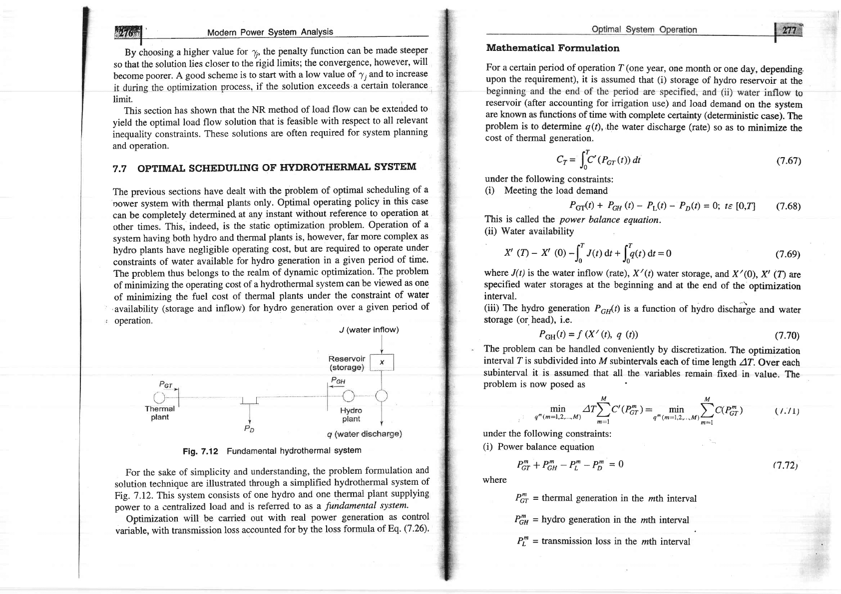
operation.
J
(water
inflow)
Fig. 7.12
Fundamental
hydrothermal
system
For the
sake
of simplicity
and
understanding,
the
problem formulation
and
solution technique
are
illustrated
through
a simplified
hydrothermal
system
of
-__----^_1--_
Q
Fig.
7 .I2.
This
system
consists
of one
hydro
and
one
thermai
piant suppiying
power to
a centralized
load
and
is referred
to as
a
fundamental
system.
Optimization
will be
carried out
with
real
power
generation as
control
variable,
with
transmission
loss accounted
for
by
the loss
formula
of
Eq.
(7.26),
Mathematical
Formulation
For
a certain
period
of
operation 7
(one
year,
one
month
or
one
day,
depending.
upon
the requirement),
it is
assumed
that
(i)
storage
of hydro
reservoir
at the
reservoir
(after
accounting
for irrigation
use) and
load
demand
on the
system
are known
as functions
of time
with complete
certainty
(deterministic
case). The
problem
is to determine q(t),,the
water
discharge
(rate)
so as
to
minimize
the
cost
of thermal
generation.
rT
Cr=
JoC
(Por(t))dt
under the
following
constraints:
(i)
Meeting
the load
demand
Pcr(r) * Pca
(t)
-
Pr(t)
-
PoG)
=
0; te
10,71
(7.68)
This is
called
the
power
balance equation.
(ii)
Water
availability
X
(T)-
x,
(o)
-l'
t@ at
+
lrqgl
dt
=o
JO
JO_
where
J(t) is the water
inflow
(rate),
X'(t) water
storage,
and
X/(0)
,
Y
(T)
arc
specified water
storages
at the
beginning
and
at the
end
of
the
optimization
interval.
(iii)
The
hydro
generation
Pcrlt)
is
a function
of
hydro
dischaige
and water
storage
(or
head), i.e.
Pcn(r)=f(X'(t),q(t))
(7.70)
The
problem
can
be handled
conveniently
by discretization.
The
optimization
interval Z
is
subdivided
into M subintervals
each of
time
length
47.
Over each
subinterval
it is assumed
that
all the
variables
remain
fixed
in
value.
The
problem
is now
posed
as
:
u^r^4-r:....*r"$^-r'(pt)
-
n^(EL
,rfrrrt,
under
the following
constraints:
(i)
Power
balance equation
Pt
*Ptr-PI-Pt
=0
where
(7.72t
Ptr
=
thermal
generation
in
the mth
interval
Ptn
=
hydro
generation
in
the
zth interval
PI
=transmission
loss in the
rnth interval
(7.67)
(7.6e)
\t.lr)
ffiffifj-
Modern Power
System
Analysis
n
n tnm t2 |
.rn
nm I D tnm t2
=
D77\r57
)
t
LDTHTGH
-f
Dpy\r6p
)
PI
=
load demand
in the mth interval
(ii)
Water continuity equation
y^
_
yt(m_r)
_
f
AT +
q^
AT
=
0
X
^
=
water
storage at the end of the mth interval
J*
--
water inflow
(rate)
in the mth interval
q^
=
water discharge
(rate)
in the ruth interval
The above equation
can be written as
Y
-
X^-r
-
J*
+
q^
=
0;
m
=
I,2, ,.., M
(7,73)
where
Y
=
X/*IAT
=
storage in discharge units.
InEqs.
(7.73),
Xo and
XM
are the
specified storages at
the
beginning
and
end
of
the
optimization interval.
(iii)
Hydro
generation
in any subinterval
Ptn
=
ho{I + o.5e
(Y
+
Y)l
(7.74)
where
ho=9.8r
x
ro-rhto
fto
=
basic
water
head
(head
corresponding to dead storage)
*
P3,
=
9.81
x
1o-2 hk@^
-,p
)
Mw
where
(q^
-
p)
=
effective discharge in m3ls
hry,
=
average head
in
the mth
interval
Now
LT(X^
+X^-r)
Optimal
System
Operation
ffiffi
l-
(7.76)
e
=
water
head correction
factor
to account
for
head
variation
with
storage
In the
above
problem
formulation,
it is convenient
to
choose
water
discharges
in
all
subintervals
except
one as independent
variables,
while
hydro genera-
tions,
thermal generations
and
water
storages
in
all subintervals
are
treated
as
dependent
variables.
The fact,
that
water
discharge
in one
of
the
subintervals
is
a dependent
variable,
is
shown
below:
Adding
Eq.
(7.73)
for
m
=
l, 2,
...,
M leads
to
the following
equation,
known
as
water
availability
equation
xM
-
"o-D
J^
+la^
=
o
(7.7s)
mm
Because
of this
equation,
only
(M
-
l)
qs
can
be specified
independently
and
the
remaining
one can then
be determined
from
this equation
and
is,
therefore,
a dependent
variable.
For
convenience, ql
is
chosen
as a
dependent
variable,
for
which
we can
write
M
qt
=
xo
-
xM
*
DJ^
-Dn^
Solution
Technique
The problem
is
solved here
using
non-linear
programming
technique
in
conjunction
with
the first
order
gradient
method.
The
Lagrangian
L
is
formulated
by
augmenting
the
cost
function
of
Eq.
(7.7L)
with
equaliry
constraints
of
Eqs.
(7
.72)-
(7.74)
through
Lagrange
multipliers (dual
variables)
\i \i'and
)i. Thus,
.c,
=D
tc(%r)
-
xT
(4r+
4,
-
ry-
ffi
+
M
(y
-
y-t-r*
+
qr)
*
^T
tp1,
-
h,
(r
+ 0.5e(y
* it11*
@^
-
p)rj (7
.77)
The dual
variables
are obtained
by equating
to
zero
the
partial
derivatives
of
the Lagrangian
with respect
to the
dependent
variables
yielding
the
following
equations
AP Ar,rDmt / rt. \
rJ)e
ut/\I
CT) ,z I n
Uf
t | ^
=
--
-Arl
l-
-
l-u
7Pt dPt
'[-
7Pt
)
0
/78)
[The
reader may
compare
this
equation
with
Eq.
(7.23)]
can
be
expressed* as
(q*
-
p)
lffi= 7ro*
2A
where
A
=
draa.
of
cross-section
of the
reservoir
at the
given
storage
h'
o
=
basic water head
(head
corresponding
to
dead storage,
hk= hLll + o.Se(x'+ X"-t)l
where
AT
Ahto
.
Now
4n=
ho
{!
+
o.Se(x^ +
x^-t)l
@^
-
P)
where
ho= 9.87
x
l0-3hto
#r,
-M-^r['-ffi)='
p
=
non:effective
discharge
(water
discharge
needed
to
run
h
dro
(7.7e)
ffil
Modern Power system
Analysis
a
(
-+)
=
)7,-
Ar*'
-
\r
p.sh"r(q*
-
p)l
-
)i*t
1o.5ho
e
I
ax^
)^**t
\/
*U
(q^
*'-
DI
-
o
and using Eq.
(7.73)
in Eq.
(7.77),
we
get
(pt-)
=
)rr- t\n"
fl
+ 0.5e
(zy
+ Jt
-
zqt
+d)=
0
(7.81)
laq' )
The dual variables for any subinterval may be
obtained
as follows:
(i)
Obtain
{
from
Eq.
(7.78).
(ii)
Obtain
)! from Eq.
(7.79).
(iii)
Obtain )1, from Eq.
(7.81)
and other
values
of
ry
(m *
1) from Eq.
'
(7.80).
The
gradient
vector is
given
by the
partial
derivatives of the Lagrangian
with
respect
to
the independent
variables.
Thus
(+)
=\f.-
^Zh"
{r
+
0.5e
(2Y-t
+
J^
-
2q^ +
p)}
(7.82)
\oq
)m+r
For
optimality
the
gradient
vector
should be zero if
there are no inequality
constraints on the control
variables.
Algorithm
Assume an initial set of independent
subintervals
except the first.
Obtain
the
values
of
dependent variables
(7.73), (7.74), (7.72)
and
(7.76).
variables
q*
(m*I)
for all
3. Obtain the dual variables
)f, \f, )i
@
=
1)
and )rr using
Eqs.
(7.78),
(739), (7.80)
and
(7.81).
4.
Obtain
the
gradient vector
using
Eq.
(7.82)
and check
if all its elements
are equal to zero within
a
specified
accuracy.
If
so,
optimum
is reached.
If
not,
go
to step 5.
5. Obtain new values of
control variables using the first
order
gradient
method,
i.e.
ek*=q;a-
{++);m=r
(7.83)
\oq* )
where
cr
is a
positive
scalar. Repeat from step 2
In the
solution
technique
presented
above, if some
of the control
variables
(water
discharges) cross the
upper or lower
bounds, these are
made equal
to
their respective bounded
values.
For
these control variables,
step
4 above
is checked
in accordance
with the Kuhn-Tucker
conditions
(7.61) given
in
Sec.
7.6.
Y, Ptu, F\r,
qt
using Eqs.
(7.80)
iently
by
augmenting
the cost
function
iith
p"nulty
functionr
ur air";;;i"
Sec. 7.6.
The
method
outlined
above
is
quite
general
and can
be
directly
extended
to
a slzstem
having
multi
has the
disadvantage
hydro
and multi-ther+nal
plan+s.
The
method,
however,
of large
memory
requirement,
since
the
independent
variables,
dependent
variables
and
gradients
need
to
be stored
simultaneously.
A
modified
technique
known
as decomposition
[24)
overcomes
this
difficulty.
In this
technique
optimization
is carried
out
over each
subinterval
and
the
complete
cycle
of iteration
is
repeated,
if
the
water
availability
equation
does.
not
check
at
the
end of
the cvcle.
Consider
the fundamental
hydrothermal
system
shown
in
Fig.
7.I2.
The
objective
is
to find
the
optimal
generation
schedule
for
a typical
dav,
wherein
load
varies
in
three
steps
of eight
hours
each
as
7
Mw,
10
Mw
and
5
Mw,
respectively.
There
is no water
inflow
into
the
reservoir
of
the
hydro plant.
The
initial
water
storage
in
the reservoir
is
100
m3/s
and
the
final
water
storage
should
be
60m3/s,
i.e. the
total
water
available
for
hydro
generation
during
the
day
is 40
m3/s.
Basic
head is
20
m. Water
head
correction
factor
e
is
given
to.be
0.005.
Assume
for
simplicity
that the
reservoir
is
rectangular
so that
e does
not
ehange
with
water
storage.
Let the
non-effective
water
discharge
be
assumed
as
2
m3/s.Incremental
fuel
cost
of the
thermal plant
is
dc
-
r.opcr
+ 25.0
Rsft'
dPcr
Further,
transmission
losses
may be neglected.
The above problem
has
been
specially
constructed (rather
ovelsimplified)
to
illustrate
the
optimal
hydrothermal
scheduling
algorithm,
which
is
otherwise
computationally
involved
and
the solution
has
to
be worked
on
the
digital
computer.
Steps
of one
complete
iteration
will
be
given
here.
Since there
are
three
subintervals,
the
control
variables
re
q2
and
q3.
Let
us
assume
their
initial
values
to
be
q2
=
75
m3ls
15 m2ls
The
value of
water diseharge
in
the first
subinterval
can be
immediateiy
found
out using
Eq.
(7.76),
i.e.
er
=
LOO
-
60
-
(15
+
15)
=
10
m3ls
It is
given
that X0
=
100 m3/s
and
X3
=
60
m3/s.
From
Eq.
(7.73)
W
Modern
po
Xt
=
f
+
Jr
-
gt
=
90 m3ls
f=Xr+12-q2=75m3/s
The values
of
hydro
generations
in the
subintervals
can be
obtained using
Eq.
(7.7q
as follows:
Pb,t=9,81
x
10-3 x20
[l
+
0.5
x
0.005
1xr
+
X0;)
{q'-
p)
=
0.1962
{I
+ 25 x
104 x
190}
x
8
=
2.315
MW
4n
=0.1962
{I
+ 25
x
lOa
x
165}
x
13
=
3.602
MW
PZa=0.1962
{l
+
25
x
10a x
135}
x
13
=
3.411
MW
The
thermal
generations
in
the three intervals
are then
pLr
=
pL- pl,
=
J
-
2.515
=
4.685 MW
4r
=
Pto- PL,
=
10
-
3.602
=
6.398 MW
Fcr=p|,-
4"
=
J
-
3.41I
=
1.589 MW
From
Eq.
(7.78),
we
have values
of )i as
dc(P€)
_
\m
ADm
-'tl
VGT
or
Calculating
),
Also
from
Eq.
From
Eq.
(7.81
\l
'
=
A\hn
ii
+
o.5e
(?)(0
+
il
-
29.685 x
0.1962
{l
+
25
-,8.474
From
Eq.
(7.E0)
for
m
=
1 and
2,
we have
^l
-zq'+ol
x
loa
(2oo
-
2o + 2)l
)T=P[,+25
for all
the three
subintervals,
we have
[^i I [2e
685]
lr?l=lrr.lsal
Lr?
j
fzo.ssrJ
(7.79),
we
can write
lril hil lzs.68s1
|
^3
|
=
|
^?
l: I
I
r:ea
I
for ttre
lossless
case
Lri
I Ld I
Lze
.sag
J
)
xt,
-
x3
-
)l
{o.Shoe
(qt
-
p)l
_
x?,
-
ll
-
^Z
{0.5
hoe
(q, _
p)l
_
Substituting
various
values,
we get
)tr=8.q14
-29.685
(0.5
x0.1962x
0.005
x
8l
_
31.398
{0.5
x
0.1962
x
0.005 x
13)
=
8.1574
)t,
=
9.1574
-
31.398 (0.5
x
0.tg6}
x
0.005
x
t3)
-
26.589 (0.5
x
0.1962
x
0.005
x
t3)
=
7.7877
Using
Eq.
(7.82),
the gradient
vector
is
(#)=
^7-
ft
n"{1
+
0.5 x
0.005
(2
x
eo
-
2 x
15
+
z)l
=
8.1574
-
31.398
x
0.1962
,{l
+
25
x
10a
x
l52l
=
-
0.3437
(
ar.l
- r3
lrf )-
A:2-
strn,
fl
+
0.5e
(2X2
+
f
-
zqt
+ p)I
lf:i=
[[]
-,'l-:::Ij
:
fli
llil
and
from
Eq.
{7.76)
4'r*=
100
-
60
-
(15.172
+
14.510)
=
10.31g
m3ls
The
above
computation
brings
us
to
the
starting
point
of
the
next
iteration.
Iterations
are
carried
out
till
the gradient
vector
U"comes
zero
within
specified
tolerance.
S!
1O.Sn"e
@,
-
p)l
=
0
)3,
1o.5ho,
(qt
-
p)]
=
o
-
7.7877
-
26.589
x
0.1962
{I
+
25 x
10a
x
t22}
=
0.9799
If
the
tolerance
fbr
gradient
vector
is
0.1,
then
optimal
conditions
are
not
yet
satisfied,
since
the gradient
vector
is
not
zero,
i.i.
(<
0.1);
hence
the
second
iteration
will
have
to
be
carried
out
starting
with
the
following
new
values
of
the
control
variables
obtained
from
Eq.
(7-g3)
lnk_l=la[,oLl#l
Lq:"*J=
L;i;l-1+l
Loq"
)
Let
us
take
a
=
0.5,
then