Kothari D.P., Nagrath I.J. Modern Power Systems Analysis

6.1

INTRODUCTION

With

the

background

of

the

we are

now

ready

to study

the

operational

features

of

a composite

power

system.

Symmetrical

steady

state

is'

in

fact,

the

most

important

mode

of

operation

of

a

power

system.

Three

major

problems

encountered

in

this

mode

of

operation

are

listed

beiow

in

their

hierarchical

order.

1.

Load

flow

problem

2.

Optimal

load

scheduling

problem

3.

Systems

control

Problem

This

chapter

is

devoted

to

the

load

flow

problem,

while

the

other

two

problems

will be

treateil

in

later

chapters.

Lt-rad

llow

study

in

power systetn

parlance

is

the

steady

state

solution

of

the

porver

system

network.

The

main

information

obtained

from

this

study

comprises

the

magnitudes

and

phase

angles

of

load

bus

voltages,

reactive

powers

at

generator

buses,

real

and

reactine

power flow

on

transmission

lines,

other

variables

being

specified.

This

information

is

essential

for

the

continuous

monitoring

of

the

current

state

of

the

systern

and

for

analyzing

the

effectiveness

of

alternative

plans for

future

system

expansion

to

meet

increased

load

demand.

Before

the

advent

of

digital

computers,

the

AC

calculating

board

was the

only

means

of

carrying

out

load

flow

studies.

These

studies

were,

therefore,

tedious

and

time

consuming.

With

the

availability

of

fast

and

large

size

digital

computers,

all

kinds

of

power system

studies,

inciuding

load

flow,

can

now be

carried

out

conveniently.

In

fact,

some

of

the

advanced

level

sophisticated

studies

which

were

almost

impossible

to

carry

out

on

the

AC

calculating

board

have

now

become

possible.

The

AC

calculating

board

has been

rendered

obsolete

for

all

practical

purposes.

6.2

NETWORK

MODEL

FORMULATION

The

load

flow

problem

has,

in fact,

been

already

introduced

in Chapter

5

with

the

help

of

a

f'undamental

systent,

i.e.

a two-bus

problem

(see

Example

5.8)'

Eor4 lq4d flqW llq4ypfufg4l

life

power system

comprising

a large

number

of buses,

it is

necessary

to

proceed

systematically

by

first

formulating

the

network

model

of

the sYstern.

A

power

system

comprises

several

buses

which

are

interconnected

by

rneans

of

transmission

lines.

Power

is

injected

into

a

bus from

generators'

while

the

loads

are

tapped

from

it.

Of

course,

there

may

be

buses

with

only

generators

and

no-loads,

and

there

may

be others

with

only

loads

and

no

generators.

Further,

VAR

generators

may

also

be

connected

to

some

buses.

The surplus

power

at some

of

the

buses

is

transported

via transmission

lines

to

buses

deficient

in

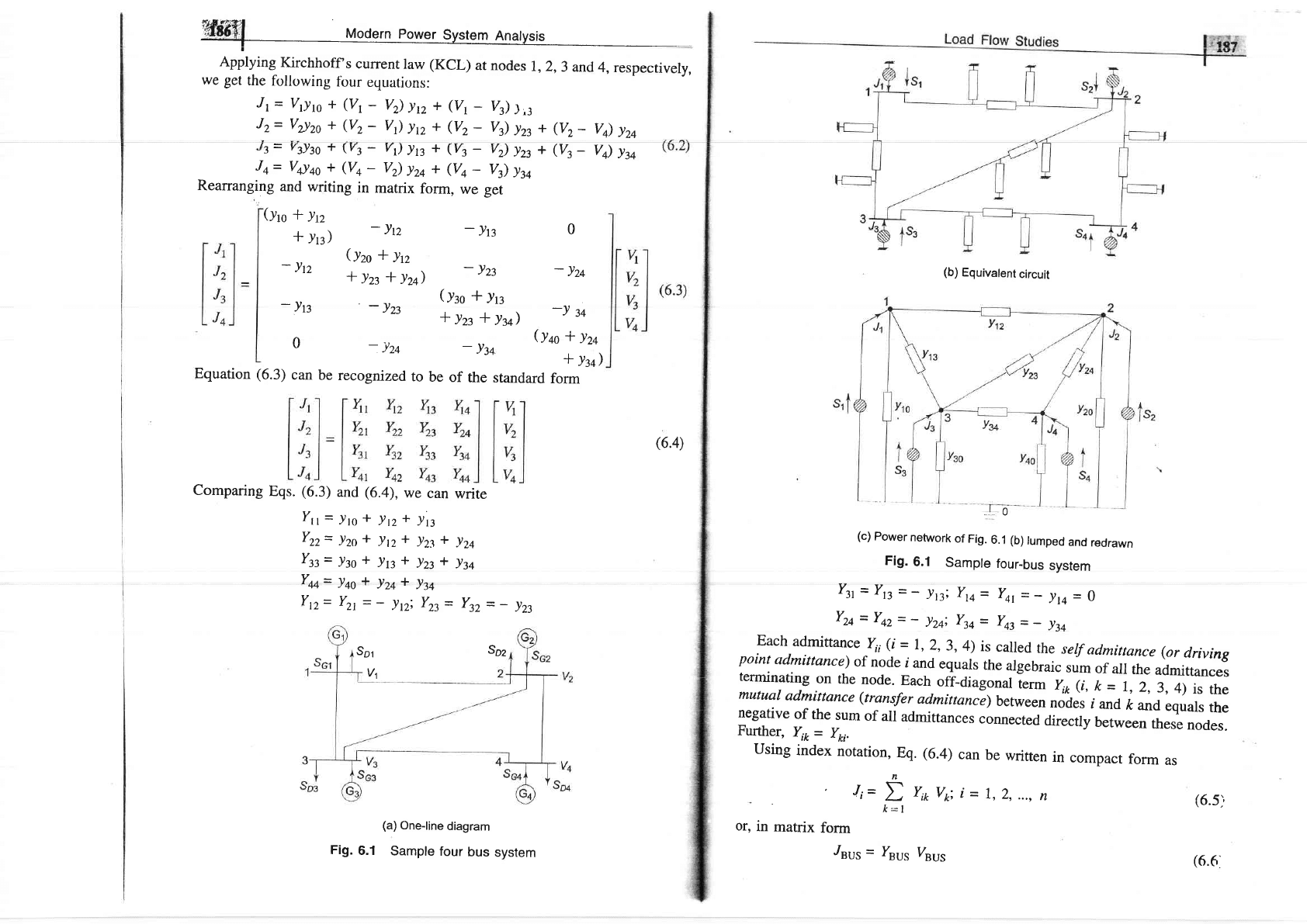
power. Figure

6.1a

shows

the

one-line

diagram

of

a

four-bus

system

with

generators

and

loads

at

each

bus.

To

arrive

at the

network

model

of

a

po*"i system,

it

is sufficiently

accurate

to

represent

a short

line by

a series

impedance

and

a long

line

by

a

nominal-zr

model.

(equivalent-7T may

be

used

foi

very

long

lines).

Often,

line

resistance

may

be

neglected

with a

small

loss

in

accuracy

but

a

great deal

of

saving

in

computation

time.

For

systematic

analysis,

it

is

convenient

to

regard

loads

as negative

generators

and lump

together

the

generator

and

load

powers

at the

buses.

Thus

at the

ith

bus,

the

net

complex

power

injected

into

the

bus

is

given

by

S;=

Pi

+

jQi= (Pci-

Po)+

j(Qci-

Qo)

where

the

corrrplex

power

supplied

by

the

generators

is

Sci=

Pot+

iQai

ancl

the

ccltnplex

power

drawn

by

the

loads

is

Spi=

Por+

iQoi

The

real

ancl

reactive

powers

injected

inttl thc

itlt

bus

arc thcn

Pi=

Poi-

P^

i

=

1,

2,

"''

fl

(6'1)

Qi=

Qci-

Qoi

Figure

6.lb

shows

the

network

model

of

the

sample

power system

prepared

on

the above

lines.

The

equivalent

power source

at

each

bus

is represented

by

a shaded

circle.

The

equivalent

power

source

at

the

ith

bus injects

current

Jr

into

the bus.

It

may

be

observed

that

the

structure

of

a

power system

is such

that

all

the

Sources

are

always

connected

to

a common

ground

node.

The

network

model

of

Fig.

6.lb

has

been

redrawn

in Fig.

6.lc

afier lurnping

the

shunt

admittances

at

the buses.

Besides

the

ground node,

it

has four

other

nocies

(buses)

at

which

the

current

from

the sources

is injected

into

the

network.

The

line

admittance

between

nodes

i and

k is

depicted

by

!ip=

Jri'Further,

the

mutual

admittance

between

lines

is

assumed

to

be

zero'

.Line

transformers

are

represented

by

tion

by

series

and

shunt

impedances,

a series

impedance

(or

for

accurate

representa-

i.e.

inverted

L-network).

apitying

Kirchhoff

s

current

law

(KCL)

at nodes

r,2,3

and

4,respectively,

we

get

the

following

fbur

equations:

Jt

=

Vrlro

+

(Vr

-

V)

ln

*

(Vr

-

Vr)

),:

Jz=

Vz)zo

+

(Vz-

Vr)

ln

+

(Vz_

V)

yzt

+

(Vz_

Vq)

yzq

s=

vztgo

+

(y:

-

v)

ln

+

(Vt

_

V)

lzz

+

(Vt_

Vq)

yzq

Jq=

Vayqo

+

(Vq

-

Vr)

lzc

*

(Vq

_

V)

yzq

Rearranging

and

writing

in

matrix

form,

we get

(yrc

*

tn

*fn,

-ln

-\z

0

.,

(lzo*ln

-

Yrz

*

hz

*

lzq,

-

lzt

-

!z+

_

!*

(y:o

*

yrg

-t23

*rzt*yy,

-lu

0

-Jz+

-

lzq

Equation

(6.3)

can

be

recognized,

to

be

of

the

standard

form

(b)

Equivalent

circuit

(c)

Power

network

of

Fig.

6.1 (b)

lumped

and

redrawn

Fig.

6.1

Sample

four-bus

system

Ylt

=

Yrc=-

lni

Yv=

Yqt

=-

)r+

=

0

Yzq=Y+z=-

lzqi

Yy=

yqz=-

ly

Each

admittance

y,,

(i

=

r,2,3,

4)

is

calred

the

serf

admittance

(or

driving

point

admittance)

of

node

i

and

equals

the

algebraic

sum

of

all

the

admittances

terminaring

on

the

node.

Each

ofi-diagonal

ierm

v*

(i,

k

=

r,

2,

3,

4)

is

the

mutual

admittance

(transfer

admittance)

between

noim

i

and

ft

and

equals

the

negative

of

the

sum

of

all

admittances

connected

directly

between

these

nodes.

Further,

Yr*

=

Yri.

using

index

notation,

Eq.

(6.a)

can

be

written

in

compact

form

as

n

Ji=

D

yp

vpi

i

=

r,2,

...,

fl

k=l

or,

in

matrix

form

"Inus

=

Isus

Vnus

(Yqa

*

yzq

*

Yz+)

Comparing

Eqs.

(6.3)

and

(6.4),

we

can

write

(6.4)

Yrr=

)ro*

ln+

ln

Yzz=

lzo

*

ltz

t

lzt

+

lzq

Ytt=

):o*

ln*

lzz*

lzq

Yu=

lqo

*

lzq

*

ly

Ytz=

Yzt

=

-

lni

YZt

=

YZZ

=

-

lZt

(a)

One-line

diagram

Fig.

6.1

Sample

four

bus

system

(6.s)

(6.6

Sor

Soz

v1

,?-blrs

system.

Furthermore,

yi*

=

0

if

buses

i

d

k

are

not

connected

(e.9.

YA

=

0).

since

in

a

power

network

each

bus

is

connected

only

to

a

few

other

buses

(usually

to

two

or

three

buses),

the

ys.y5

of

a

rarge

network

is

very

sparse'

i'e'

it

has

a

large

number

of

zero

elementi.-itrougtr

tf,i,

prop"rty

is

not

evident

in

a

small

system

like

the

sample

system

under

consideration,

in

a

system

containing

hundreds

of

buses,

the

sparsity

may

be

as

high

as

90vo.

Tinney

and

associates

[22]

at

Bonnevile

Power

Authority

were

the

first

to

exploit

the

sparsity

feature

of

zsu5

in

greatly

reducing

numerical

computations

in

load

flow

studies

and

in

minimizing

the

memory

required

as

only

non-zero

terms

need

be

stored.

Equation

(6.6)

can

also

be

written

in

the

form

urhanp V J^-^+^^ aL^ -- ^^ :

'vrrvrv

-BUS

\re,'ulsD

urc

llralnx

or

DUS

admlttance

and

is

known

as

bus

admittance

matrix.

The

dimension

of

the

y"u5

matrix

is

(n

x

n)

where

n

is

the

number

of

buses'

[The

total

number

of

nocles

ii e

m

=

n +

|

including

the ground

(reference)

node.l

As

seen

above,

yru,

is

a

symmetric

except

when

phase

shifting

transformers

are

involved,

so

that

only

nv+

t)

terms

are

to

be

stored

for

an

2

1.,.^L{"

involved

algorithms.

Furthermore,

the

impedance

matrix

is

a

fuil

matrix.**

The

bus

impedance

matrix,

however,

is

most

useful

for

short

circuit

studies

as

will

be

seen

in

Chapters

10

and

11.

Note:

In

the

sample

system

of

Fig.

6.1.

the

arDrrrary

manner,

although

in

more

sophisticated

studies

of

large

power

systems,

it

has

been

shown

that

certain

ordering

of

nodes

produfes

faster

convergence

and

solutions.

Appendix

c

deals

with

the

topics

of

sparsity

and

optimal

ordering.

6.3

FORMATION

OF

fsus

BY

SINGULAR

TRANSFORMATION

Graph

Vnus

=

Zausleus

where

Zsu5

(bus

impedance

matrix)

=

fsLs

fbr

a

network

of

fbur

buses (fbur

inclependent

nodes)

(6.7)

(6.8)

-flmmetric

rnus

yields

symmetric

Zsus.

The

diagonal

erements

of

Zuu,

are

called

driving

point

imped,ances

of

the

nodes,

and

th!

off-diagonal

elements

are

called

transfer

impedances

of

the

nodes.

Zsus

need

not

be

obtained

by

inverting

rnus.while

y"u,

is

a

sparse

matrix,-Auris

a

full

matrix.

i.e.,

zero

elements

of

I'ru,

become

non-zero

in

the

.o,,.rp"o"niing

Zsu,

erements.

It

is t'

be

stressed

here

that

yBus/zBus

constitute

models

of

the

passive

portions

of

the power

network.

Bus

admittance

matrix

is

often

used

in

sorving

road

flow problem.

It

hal

gained

widespread

application

owing

to

its

simpticity

of

data preparation

and

the

ease

with

which

the

bus

admittance

matrix

can

be

formed

ano

moOfied

for

network

changes-addition

of

lines,

regulating

transformers,

etc.

(see

Examples

6'2

and6'7)'

of

course,

sparsity

is

one

of

its greatest

advantages

as

it

heavily

reduces

computer'memory

and

time

requirernents.

In

contrast

to

this,

the

zss"

can

be

referred

to ground

or

slack

bus.

In

the

former

case,

it

is

usually

necessary

l'o

creal'e

at

least

one

strong

artificial

tie

to ground

to

avoid

numerical

difficulties

when

obtaining

Zsg5,

because

in

absence

of

this,

rr*

is

ilr-conditioned

or

even

singular'

A

large

shunt

admittance

inserted

at

the

slack

bus

most

simply

achieves

the

desired

result

[20].

**The

disadvantages

of

the

conventional

impedance

matrix

may

be

overcome

by

making

use

of

LU

factors

of the

admittance

matrix

and

bf

employing

compacr

srorage

scheme'

Piecewise

methods

or tearing

techniques

(dialoptics)

have

recently

been

applied

to

overcome

the

disadvantages

of

excessiv,

,rorug.

requirements

Ilg].

***For

convenience,

direction

is

so

assigned

as

to

coincide

with

the

assu'red

positive

direction

of

the

element

current.

i90

l

Modern

power

System

Anatysis

Or@

o

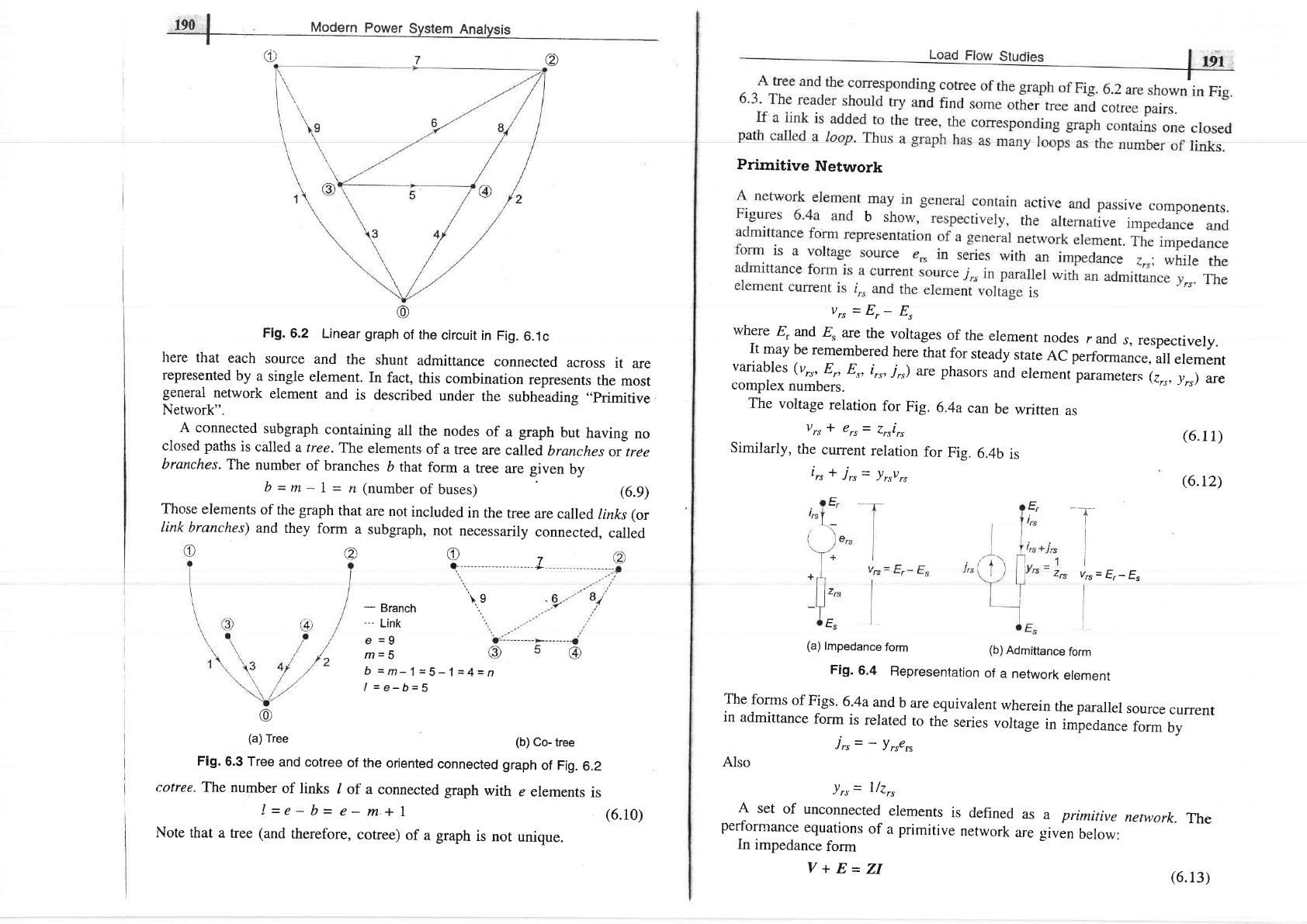
Fig.

6.2

Linear

graph

of the

circuit

in Fig.

6.1c

here

that

each

source

and

the

shunt

admittance

connected

across

it

are

represented

by

a single

element.

In

fact,

this

combination

represents

the

most

general

network

element

and

is

described

under

the

subheading

"primitive

Network".

A

connected

s'bgraph

containing

all

the

nodes

of

a

graph

but

having

no

closed

paths

is

called

a tree.

The

elements

of a

tree

are called

branches

or ffee

branches.

The

number

of branches

b

that

form

a

tree

are given

by

b=m

*

1-

n

(numberof

buses)

(6.9)

Those

elements

of

the

graph

that

are

not

included

in

the

tree

are

called

links

(or

link

branches)

and

they

form

a

subgraph,

not

necessarily

connected,

called

-

Branch

-

Link

e

=9

m=5

b=m-1=5-'l=4=n

l=e-b=5

@

(a)

Tree

(b)

Co- tree

Fig.

6.3 Tree

and

cotree

of the

oriented

connected graph

of Fig.

6.2

cotree.

The number

of links

/

of

a connected

graph

with

e

elements

is

I=e-b=e-m+l

Note

that

a tree

(and

therefbre,

cotree)

of

a

graph

is

not

unique.

Primitive

Network

vr,

=

Er-

E,

where

E,

and

E"

are

the

voltages

of

the

element

nodes

r

and

s,

respectively.

It

may

be

remembered

here

that

for

steady

state

AC performan..,

ull

element

variables

(vr*

E,

8",

irr,7r.,)

are phasors

and

element

parameters

(zrr,

.rr")

ar€

complex

numbers.

The

voltage

relation

for

Fig.

6.4a

can

be

written

as

vrr*

€rr=

Zrri^

Similarly,

the

current

relation

for

Fig.

6.4b

is

ir,

*

jr, =

lrrv^

(a)

lmpedance

form

(b)

Admittance

form

(6.11)

(6.r2)

rn

v7

o-------------

- --------+

\.e

@

c

!r.,=

|/7r,

A

set

of

unconnected

elements

is

defined

as

performance

equations

of

a primitive

network

erre

In

impedance

form

I

yr"=E

-E"

a primitive

network.

The

given

below:

Fig.

6.4

Representation

of

a

network

element

The

forms

of

Figs.

6.4a

and,

b

are

equivalent

wherein

the

parallel

source

currenr

in

admittance

form

is

the

series

voltage

in

impedance

form

by

Jr,=

-

Yrs€rs

Also

(6.10)

V+E=ZI

(6.13)

'f{W';l

Modern

Power

svstem Anatvsis

In

admittance

form

I+J=W

(6.14)

Load

Fiow

Stucjies

i

flH:

<

v

=

AV,'J'

I

(6.16)

where

the

bus

incidence

matrix

A

is

Here

V and.I

are

the element

voltage

and

current

vectors

respectively,

and

rl

and

E

are the

source vectors.

z and

Y are

referred

to as

the

primitive

i

admittance

matrices,

respectively.'These

are

Z

=

Y-r.If

there

is no

mutual

coupling

between

elements,

Z

and

Y are

diagonal

where

the

diagonal

entries

are

the

impedances/admittances

of

the network

elements

and

are

reciprocal.

NeturorkVariables

in Bus

Frame

of Reference

Linear

network graph

helps

in the

systematic

assembly

of a network

model.

The

main

problem

in

deriving

mathematical

models

for large

and

complex power

networks

is

to select

a

minimum

or zero

redundancy (linearly

independent)

set

of

current

or voltage

variables

which

is sufficient

to

give

the

information

about

all

element

voltages

and

currents.

One

set

of such

variables

is

the

b tree

voltages.*

It

may easily

be seen

by

using

topological

reasoning

that

these

variables

constitute

a non-redundant

set. The

knowledge

of b

tree

voltages

allows

us

to compute

all

element

voltages

and therefore,

all

bus

currents

assuming

all element

admittances

being

known.

Consider

a

tree

graph

shown

in

Fig.

6.3a where

the ground

node

is

chosen

as

the reference

node.

This

is the

most

appropriate

tree

choice

for

a

power

network.

With

this

choice,

the

b

tree

branch

voltages

become

identical

with

the

bus voltages

as

the tree

branches

are

incident

to

the

ground

node.

Bus

Incidence

Matrix

For

the

specific

system

of Fig.

6.3a,

we

obtain

the

following

relations

tetween

the

nine

element voltages

and

the four

bus

(i.e.

tree

branch)

voltages

V1,

V2, V3

and Va.

Vut

=

Vt

Vtz=

Vz

Vut

=

Vt

Vuq=

Vq

Vts=

Vt-

Vta=

Vt

-

Vn=Vt-

Vts=

Vq-

Vtg=

Vt-

or,

in matrix

form

*Another

useful

set

of

network

variables

are

the

/ link

(loop)

currents which

constitute

a zero

redundancy

set

of network

variables

[6].

1000

0100

0010

0001

001_l

0-l

10

l-l

00

0-1

01

-l

010

This

matrix

is

rectangular

and

therefore

singular.

as per

the

following

rules:

e

I

2

3

4

)

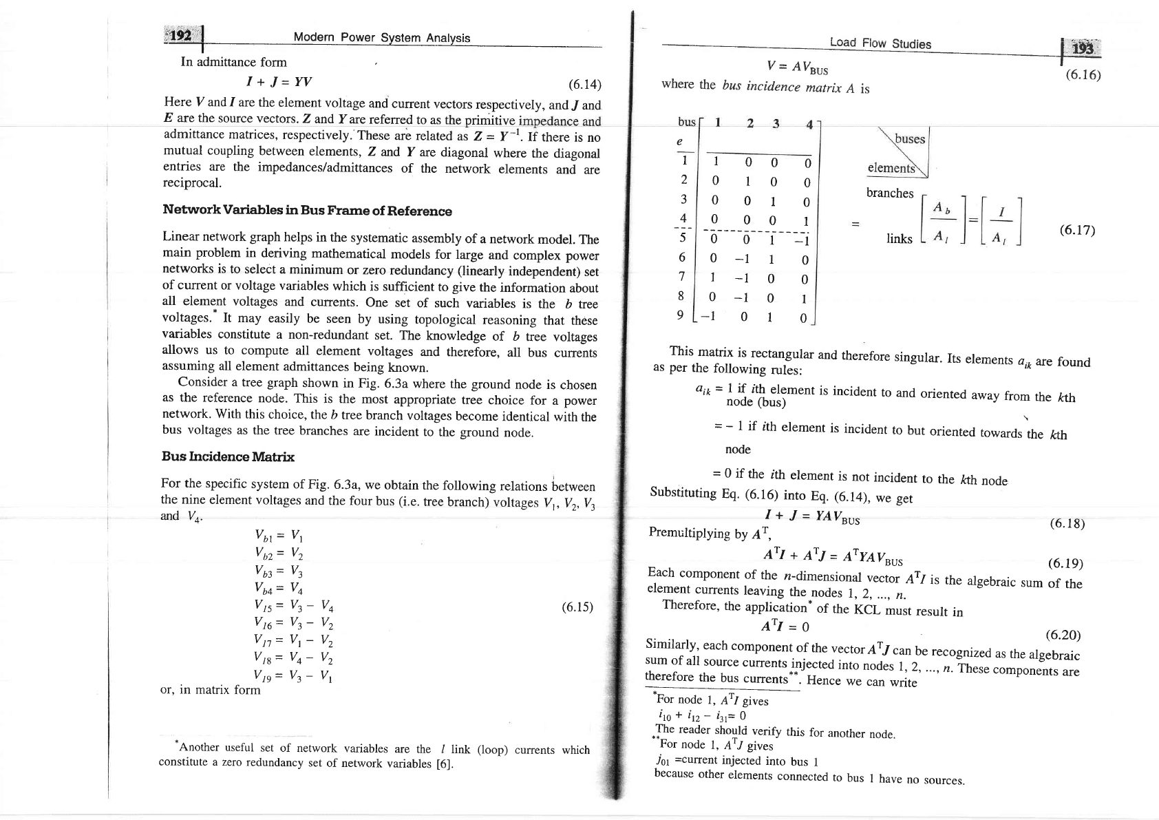
6

7

branches

links

8

9

(6.r7)

Its

elements

a,oare

found

and

oriented

away

from

the

ftth

to

but

oriented

towards

the

ftth

aik

=

1 if

tth

element

is

incident

to

node (bus)

=

-

|

if

tth

element

is

incident

node

=

0 if

the

ith

element

is

not

incident

to

the

kth

node

Substituting

Eq.

(6.16)

into

Eq. (6.14),

we

get

I+J=yAVsu5

Premultiplying

by

Ar,

ArI+ArJ=AryAV"u,

F,ach

component

of

the

n-dimensional

vector

ATI

is

the

element

currents

leaving

the

nodes

7,2,

...,

n.

Therefore,

the

application*

of

the

KCL

must

result

in

ArI

=o

(6.20)

Similarly,

each

component

of

the

vector

ATJ

"unbe

recognized

as

the

algebraic

sum

of

all

source

currentsinjected

into

nodes

r,2,

...,n.

These

components

are

therefore

the

bus

currents**.

Hence

we

can

write

*For

node

l,

Arl gives

iro

+

ir,

-

l:r=

0

-The

reader

shoulci

verify

this

for

another

node.

**For

node

l,

AT"/ gives

j61

=current

injected

into

bus

1

because

other

elements

connected

to

bus

t

have

no

sources.

(6.

l8)

(6.1e)

algebraic

sum

of

the

Vn

v2

vr

(6.15)

i,il9:4iitl

Modern

Power Svstem Analvsis

- .

-

J

- ---- - -"--'f

---

I

ArJ

=

Jsus

Equation

(6.19)

then is

simplified

to

,/eus

=

ATYAV",,,,

--J---.^^_-.--rr^'vrrrrgvl'va

the same nodal

current

equation

as

(6.6).

The

bus admittance

matrix can

then

be obtained

from the

singular

transformation

of the

primitive

Y, i.e.

Yeus

=

ATYA

Load

Flow

Studies

I ftt^

I

v

-

lTv,r

rBUS

=

A IA

(6.2r)

(6.22)

(6.23)

0

-

!'tn

A

computer programme

can

be developed

to

write the

bus incidence

matrix

A

from

the

interconnection

data of

the directed

elements

of the

power

systetn.

Standard matrix

transpose

and multiplication

subroutines

can

then be used to

compute

Yu*

fiorn Eq.

(6.23).

*"*'^-"r

,

Example

6.1

|

I

Find the

Y6u"

using singular

transformation

for the

system

of

Fig.

6.2.

Solution

Y-

Using A fiom

*

yr:)

(yzo

*

yn

-

Jtz

*

lzt

*

t-zq,

-

lzt

-

)r:

,.

()'lo

f-

.yr

'-

.t'23

*

lzt

*

Jy,

-

}'l

0

_!zc

The

elements

of this

matrix,

of course,

agree

with

those

previously

calculated

in

Eq.

(6.3)

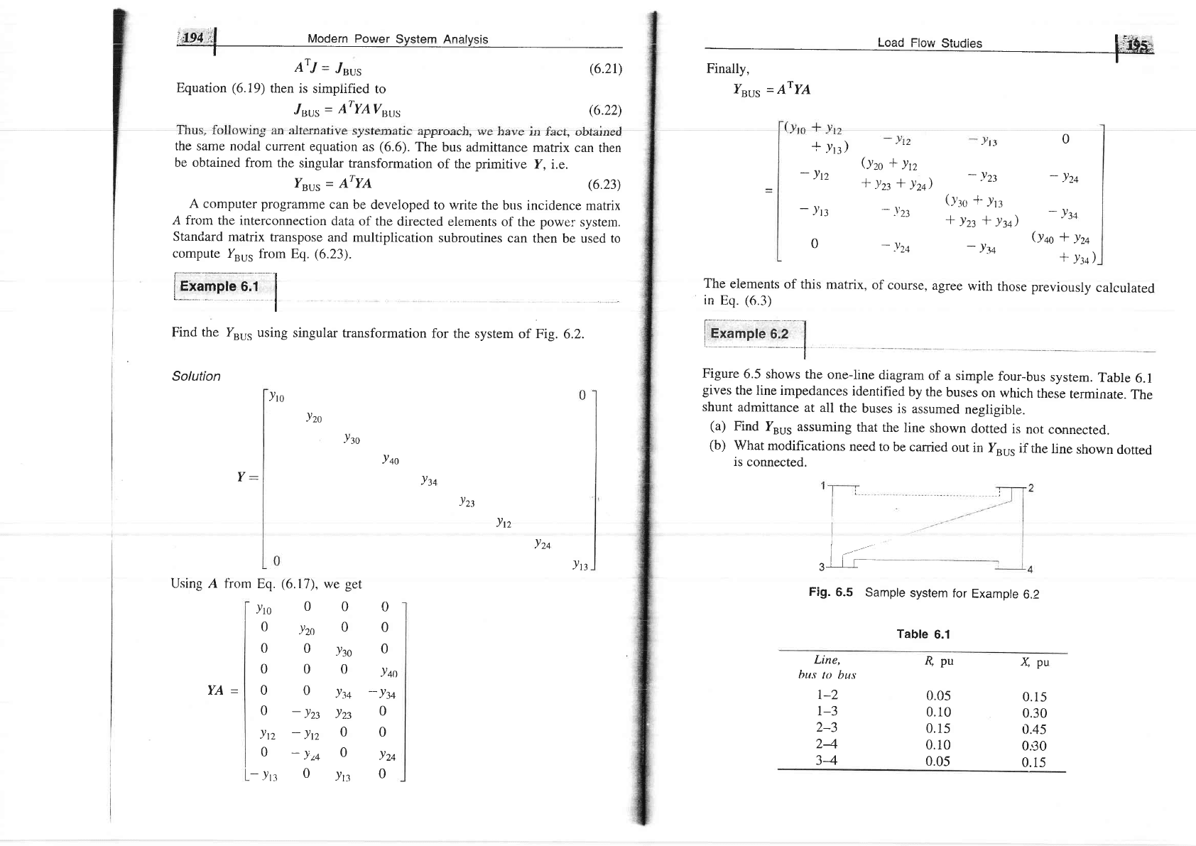
)ro

Figure

6.5

shows the

one-line

diagram

of

a simple

four-bus

system.

Table

6.1

gives

the

line impedances

identified

by

the

buses

on which

these

terminate.

The

shunt

admittance

at all

the

buses

is

assumed

negligible.

(a)

Find

Yuu.

assuming

that

the

line

shown

dotted

is

not

connected.

(b)

What

modifications

need

to

be carried

out

in

Yuu,

if

the

line

shown

dotted

is

connected.

Fig.

6.5

Sample

system

for

Example

6.2

Table

6.1

!zo

-Vro

!qo

ltn

v-,

JZ)

!n

Y.-n

ln

IJ1'

3

Eq.

)ro

0

!n

0

-.Yrr

0

jqo

-

ft+

0

lzq

0

&pu

0.05

0.10

0.15

0.10

0.05

xpu

0.15

0.30

0.45

0.E0

0.15

(6.17),

we

get

00

lzo

0

0Jn

00

0ly

-

jzz

lzz

-lrz

0

-

!24

0

0ln

Line,

bus

to bus

t-2

1-3

2-3

24

34

YA=

trrrr.F,b"iFl

'f|/0.!:l

Modern

Power

Svstem Anatvcis

-t

Table

6.2

f.siffi

where

V, is the voltage at the ith bus with

respect to

ground

and

,/,

is the

source

current injected into the bus.

The load flow

problem

is handled

more conveniently

by use

of

"/,

rather

than

,I,t. Therefore, taking the complex conjugate

of Eq.

(6.24),

we

have

(6.25a)

Substituting for

J,

=

Y*Vr from

Eq.

(6.5),

we can write

Line

r-2

Gpu

2.0

1.0

2.0

B,pu

-

6.0

-

J.\,

-

2.0

-

3.0

-

6.0

2-3

24

34

t

k:l

solution (a)

From

Table

6.1,

Table

6.2

is

obtained

from

which

yuu,

for

the

system

can

be written

as

added

between

buses

7 and

2.

Ytz,

n"*

=

Yrz,

on

-

(2

-

j6) =

Yzr.

o"*

Xrr,

n"*

=

ytt,ora

+

(2

-

j6)

(iv)

Y2z,

n"*

=

Yzz,

ot,t

+

(2

-

j6)

Modified

Y"u,

is

written

below

6.4 LOAD

FLOW

PROBLEM

The

complex

power

injected

by

the

source

into

the

ith

bus

of

a

power

sysrem

IS

Qi

(reactive

power)

=

-

Irn

In

polar

form

V;

=

ll/,1si6t

Y

r*

=

lY'ol eio'r

Real and reactive

powers

can now be expressed

as

n

P,

(real

power)

=

lvil

D

lvkl lYikl cos

(0,0

+

k:l

i= r,

A

Pi-

jQi=Vf

L

Yil,Vpi

k:l

Equating real and imaginary

parts

I

P;

(real

power)

=

Re

]Vi

t

i=l2 n

(6.2sb)

(6.26a)

(6.26b)

(6.27)

6,);

(6.28)

6t

-

6');

2,

..., fl

Qi Qeactive

power)

-

lvil

D

lvkl lYikl sin

(e,1

+

6t

-

k:l

i=1,2,...,fl

Equations

(6.27)

and

(6.28)

represent 2n

power

flow equations

at

n

buses

of

a

power

system

(n

real

power

flow equations and

n reactive

power

flow

equations). Each bus is

characterized

by four variables;

P;,

Qi,

l7,l

and

6i

resulting in a total of

4n variables.

Equations

(6.27)

and

(6.28)

can be

solved

for 2n

variables

if

the remaining 2n

variables

are specified. Practical

considerations

allow a

power

system analyst

to fix a

priori

two

variables

at

each bus. The

solution for

the remaining

2n bus variables

is rendered difficult

by the fact

that Eqs.

(6.27)

and

(6.28)

are non-linear

algebraic

equations

(bus

voltages

are

involved in

product

form and

sine and cosine

terms are

present)

and therefore,

explicit solution

is not

possible.

Solution can

only be

obtained

by

iterative numerical

techniques.

(6.24)

:flg.,0iil

toaern

power

system

Anatvsis

Depending

upon

which

two

variables

are

specified

a

priori,

the

buses

are

classified

into

three

categories.

(I)

PQ

Bus

r rr

rrrro

rJyw

vr

LruD,

Lrrc

ucr

puwers

ri

ano

ai

arc

known

(po,

and

Qpi

arc

known

l."l 1:1t"t:i:.t"

g

ancl

p,

and

egile

specified).

The

*tnn*i,

ars

f

l/,t

and

6,. A

pure

load

bus

(no

generating

f*ifty-at

the

bus,

i.e.,

pcr=

eci=0)

is

a

Pp

bus.

(2)

PV

Bus/Generator

Bus/voltagre

controlled

Bus

At this

type

of

bus

P'

and

eo,

are

known

a

priori

and

rv,r

and.

p,(hence

p6;)

are

specified.

The

unknowns

are

e,

(hence

eo,)

and

6,.

'

\

(3)

Slack

Bus/Swing

Bus/Reference

Bus

state

variables.

These

adjustable

independent

variables

are

called

control

parameters.

Vector

J

can

then

be

partitioned

into

a

vector

u

of

confrol

parameters

and

a vector p

of fixed parameters.

In

a

load

flow

study

real

and

reactive

powers

(i.e.

complex

power)

cannot

be fixed

a priori

at

alr

the

buses

as

the

net

complex

power

flow

into

the

network

is

not

known

in

advance,

the

system

power

loss

being

unknown

till

the

load

flow

study

is

complete.

It

is,

therefore,

n.."rrury

to

have

one

bus

(i.e.

the

slack

bus)

at

which

complex

power

is unspecified

so

that

it

supplies

the

difference

in

the

total

system

load

plus

losses

and

the

sum

of

the

complex

powers

specified

at

the

rcrnaining

buses.

By

the

same

reasoning

the

slack

bus

must

be

a

generator

bus.

The

complex

power

allocated

to

this

bus

is

determined

as

part

of

the

solution.

In

order

that

the

variations

in

real

and

reactive

powers

of the

slack

bus

during

the

iterative

process

be

a

snrall

percentage

of

its

generating

capacity,

the

bus

connectecl

to

the

largest

generating

station

is

normally

selected

as

the

slack

bus.

Further,

for

corivenience

the

slack

bus

is

numbered

as

bus

1.

Equations (6.27)

and

(6.28)

are

referred

to

as

stutic

load

ftow

equations

(SLFE)'

By

transposing

all

the

variables

on

one

side.

these

equations

can

be

written

in

the

vector

form

f(x,y)-o

,f

=

vector

function

of

dimension

2n

x

=

d_ependent

or

state

vector

of

dimen

sion

2n

(2n

unspecified

variables)

Control parameters

may

be voltage

magnitudes

at

pV

buses,

real powers

p,,

etc.

The

vector p

includes

all the

remaining

parameters

which

are

uncontrollable.

For SLFE

solution

to

have

practical

significance,

all

the

state

and

control

variables

must

lie within

specified practical

limits.

These

limits,

which are

dictated

by

specifications

of

power

system

hardware

and

operating

constraints,

are

described

below:

(i)

Voltage

magnirude

lV,l

must

satisfy

the

inequality

lv,l^tn

<

lvil

(

lv,l_*

(6.31)

The

power

system

equipment

is

designed

to

operate

at

fixed

voltages

with

allowable

variations

of t

(5

-

l})Vo

of

the

rated

values.

(ii)

Certain

of the

6,s

(state

variables)

must

satisfy

the

inequality

constraint

16,-

6ft1

S

l6i-

6rln,o

(6.32)

This

constraint

limits

the

maximum permissible

power

angle

of transmission

line connecting

buses

i and

ft and

is

imposed

by

considerations

of

system

stability

(see

Chapter

12).

\

-

(iii)

owing

to

physical

limitations

of

p

and/or

e

generation

sources,

po,

and

Qci

Ne

constrained

as

follows:

(6.30)

(6.33)

(6.34)

(6.35)

(6.36)

Pc,,

^in

1

Pc,

S

Pc,.

,n*

Qci,

^rn

1

Qci S

Qc,,

^u**

(6.2e)

It

is, of

course,

obvious

that

the

total

generation

of real

and

reactive

power

must

equal

the

total

load demand plus

losses,

i.e.

D

Po,=t

Po,+

P,

lt

D

Qci=l

Qot+

Qr

ii

where

Ptand

Qpare

system

real

and

reactive power

loss,

respectively.

Optimal

sharing

of active

and reactive

power

generation

between

sources

will be

discussed

in

Chapter

7.

-Voltage

ata

PV

bus can

be

maintained

constant

only

if conrollable

esource

is

available at

the bus

and

the

reactive generation

required

is within

prescribed

limits.

where

)

=

vector

of

independent

variables

of

dimension

2n

(2n

independent

variabres

which

are

specified.

i prrori)

ffi#ilfl,.l.i|

Mod".n

Po*"t

sv"ttt

An"lvtit

I

"Ihe

load

flow

problem

can

now

be

fully

defined

as follows:

Assume

a

certain

nominal

bus

load

configuration.

Specify

P6i+

iQci

at all

the

pQbuses

(this

specifies

P,

+

iQi

at

these

buses);

specify

Pcr

(this

specifies

P,)

and

lV,l

at all

the

PV buses.

Also

specify

lVll

and

6,

(=

0)

at the

slack

bus'

T.L,,- r- .,--iolrlac nf thp rrer-fnr u ere snecifie.d The 2n SLFE can now be

solved

(iteratively)

to

determine

the

values

of

the

2n

vanables

of

the

vector

x

comprising

voltages

and

angles

at the

PQ buses,

reactive

powers and

angles

at

fhe

pV

buses

and

active

and

reactive

powers

at the

slack

bus.

The

step

is

to

comPute

line

flows.'

So

far

we have

presented,

the

methods

of assembling

a Yeus

matrix

and

load

flow

equations

and

have

defined

the

load

flow

problern

in its

genpral form

with

definitions

of

various

types

of

buses.

It

has been

demonstrated

that

load

flow

equations,

being

essentially

non-linear

algebraic

equations,

have

to be

solved

through

iterative

numerical

techniques.

Section

6.5

presents

some

of the

algorithms

which

are

used

for

load

flow

solutions

of

acceptable

accuracy

for

systems

of

practical

size.

At

the

cost

of

solution

accuracy,

it is

possible

to linearize

load flo-w

equations

by

making

suitable

assumptions

and

approximations

so

that

f'ast

and

eiplicit

solutions

become

possible.

Such

techniques

have

value

particularly for

planning

studies,

where

load

flow

solutions

have

to

be carried

out

repeatedly

but

a

high

degree

of

accuracy

is not

needed.

An

Approximate

Load

Flow

Solution

Let

us

make

the

following

assumptions

and

approximations

in the

load

flow

Eqs.

(6.27)

and

(6.28).

'

(i) Line

resistances

being

smaii

are

rreglecie,C

(shiint conductance

of overhead

lines

is always

negligible),

i.e.

P7,

the

active

power loss

of

the system

is

zero.

Thus

in

Eqs.

(6'21)

and

(6.28)

1it

=

90'

and

1ii

-

90o

'

(ii)

(6,

-

6r)

is small

(<

r/6)

so

that

sin

(6,

-

6o)

=

(6r

-

6r).

This

is

justified

from

considerations

of

stability

(see

Chapter

72)'

(iii) AII

buses

other

than

the

slack

bus

(numbered

as

bus

1) are

PV

buses,

i.e.

voltage

magnitucles

at

all the

buses

including

the

slack

bus

are

specified.

Equations

(6.27)

and

(6.28)

then

reduce

to

Pi

=lVil

lvkl

lYikl

(6i

-

6r);

i

=

2,3,

...,

n

(6.37)

n

et=-

'u,'

E

rvkrlyikr

cos

(6,-

6u)

+rv,r2

ry,,r;

i

=

r,2,...,

n

(6.39)

Since

lv,ls

are

specified,

Eq.

(6.37)

represents

a set

of

linear

algebraic

equationi

in 6,s

r,vhich

are

(n

-

l)

in

number

as

6,

is

specified

at the

slack

bus

(6,

=

0).

The

nth

equation

corresponding

to

slack

bus

(n

=

l)

is

redundant

as

the

reat

power

injected

at this

bus

is now

fully

specified

as

Wffi

nn

Pr

=

.I

Po,-

D

Po,; (Pr=

0).

Equations

(6.37)

can

be

solved

explicirly

i:2

(non-iteratively)

for

62,

61,

...,

d,

which,

when

substituted

in

Eq.

(6.3g),

yields

madehaveo..ouiLii*i;:;ffi

,"(;:;'iLT,",",T:,:T:J"#il-,1',T,7

simultaneously

but

can

be

solved

sequentially

[solution

of

Eq.

(6.3g)

follows

immediately

upon

simurtaneous

sorution

of

Eq.

(6.37)).

Since

the

sorution

is

non-iterative

and

the

dimension

is

retlucecr

to

(rr-l)

from

Zrt,

it

is

computationally

highly

economical.

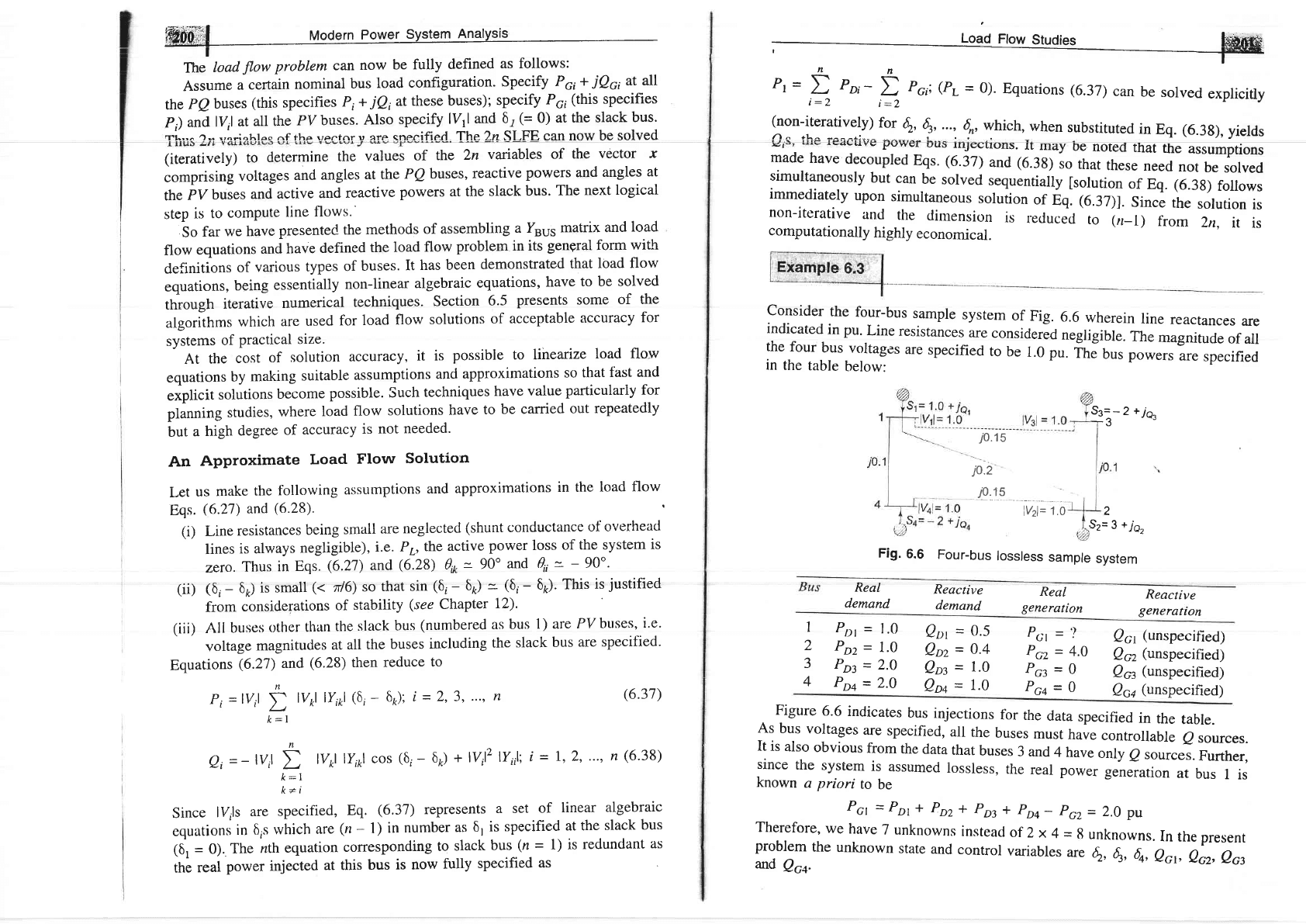
consider

the

four-bus

sample

system

of

Fig.

6.6

wherein

line

reactances

are

indicated

in pu.

Line

resistances

are

considerld

negligible.

The

magnitude

of

all

the

four

bus

vortages

are

specified

to

be

r.0 pu.

itJuu,

powersLe

specified

in

the

table

below:

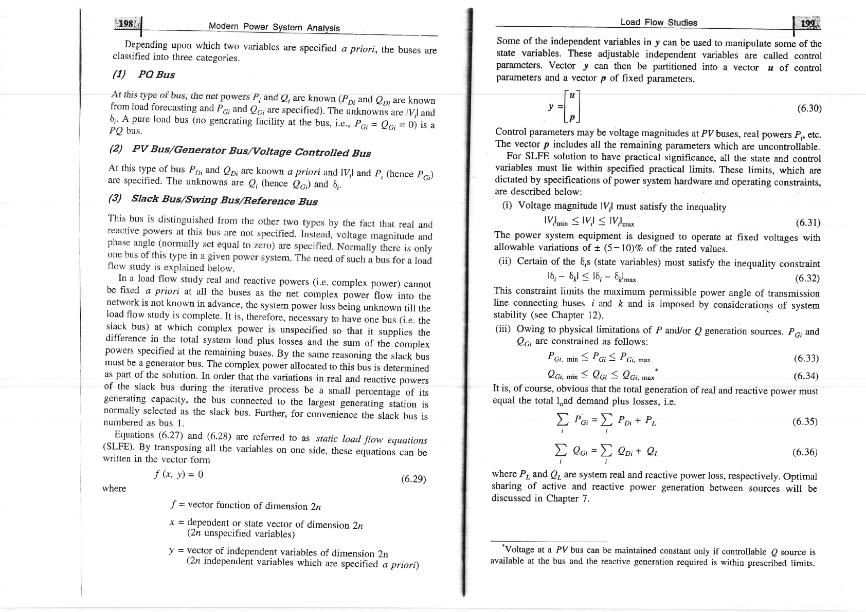
53=-

2

+7O,

--r

J

j0.15

jo.2

iP,ts

lVzl=

'l.o

.S.= I + i^

,,-.

-

I

Uz

Fig.

6.6

Four-bus

lossless

sample

system

2

Real

demand

Reactive

demand

Real

generation

Reactive

generatrcn

1

2

3

4

Por

=

1.0

Qot

=

0.5

Poz

=

7.0

Qoz

=

0.4

Poz

=

2.0

Qoz

=

1.0

Poq

=

2.0

Qoq

=

7.0

061

(unspecified)

Q62

(unspecified)

O63

(unspecified)

06a

(unspecified)

Pcl

='-

Pcz

=

4'0

Pct=o

Pcq=o

n

\-

,/--r

k:1

Figure

6.6

indicates

bus

injections

fbr

the

data

specified

in

the

table.

As

bus

voltages

are

specified,

all

the

buses

must

have

controllable

e

sources.

Il_r::t::

"_bviyus

from

the

data

rhar

buses

3

and

4

have

onry

e

sources.

Further,

slnce

ffie

system

is

assumeci

lossless,

the

real

power

generation

at

bus

I

is

known

a

priori

to

be

Pct

=

Por

*

Poz

*

pot

*

poo_

pcz

=

2.0

pu

Therefore,

we

have

7

unknowns

instead

of

2

x

4

=

8

unknowns.

In

the

present

problem

the

unknown

state

and

control

variables

are

{,

e,

60,

ect,

ecz,

ecz

and

Qc+.

Using

the

above

Y"u,

and bus

powers

as shown in Fig. 6.6, approximate

load

flow Eqs.

(6.37)

are

expressed

as

(all

voltage

magnitudes

are equal to 1.0

pu)

'yili.\

Modern Power System Analysis

I

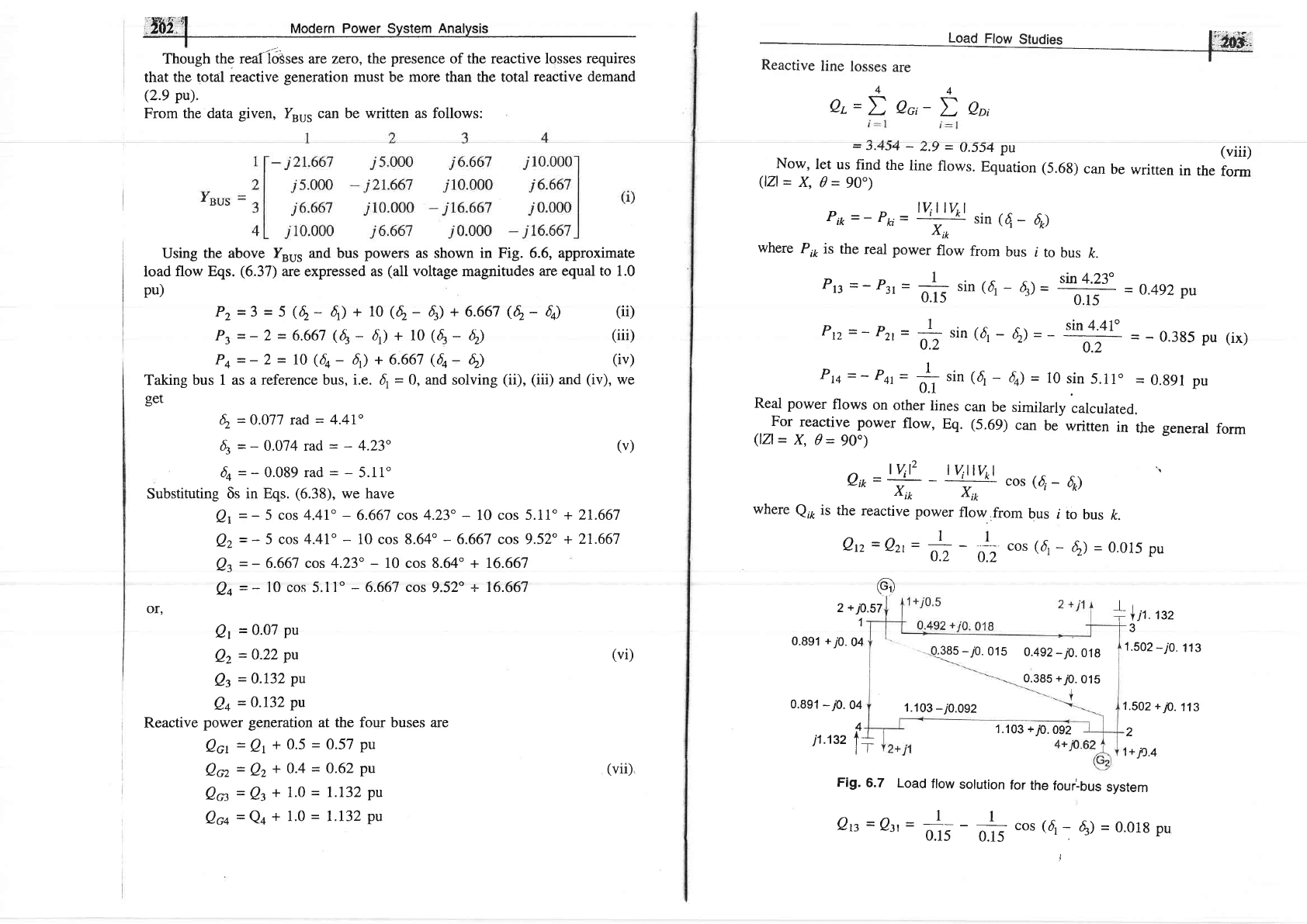
Though the

reali63ses

are

zero, the

presence

of the reactive losses requires

that

the total reactive

generation

must be more than the total

reactive demand

(2.9

pu).

From the data

given,

Yru5 can be written as follows:

44

er=D

eo,-

D

epi

_

r.+r+

_

L,>

=

u.JJ4 pu

(viii)

Now,

let

us

find

the

line

flows.

Equation

(5.6g)

can

be

written

in

the

form

(lzl=

X,0=90")

2

+ j0.ET

1

3

0.891

+/O.

04

0.891

-7O.

04

,385

-70.

015

0.492

-70.

018

0.385

+,p.

01S

1.s02

-i0.

113

1.502

+

10.

113

2

t,

jD.4

1.103

-

j0.0s2

4

1.103

+p.

092

Pz= 3

=

5

(6-

6)

+ 10

(6-

4)

+

6.667

(6-

6q)

Pt

=-

2

-

6.667

(6-

4)

+ l0

(4

-

6)

P+=-2- 10(4-

4)

+6.667

(6q:6)

Pik

=

-

Pki

-

lvi]-lvkl

sin

({

-

6o)

x,o

where

P*

is

the

real

power

flow

from

bus

j

to

bus

k.

pn

=

-

pz,

=

+

sin

(d,

-

q)-

sin-1.23"

=

0.492

pu

0.15

\r

-r/

0.1:

Ptz

=

-

Pzr

=

-1-

sin

(4

-

6)

=

- $n

4'41o

L'L

0.2

02

=

-

0'385

Pu

(ix)

Pru=-

Pqt=

+

sin

({

-

6o)

=

10

sin

5.11o

=

0.g91

pu

0.1

Real power

flows

on

other

lines

can

be

similarly

calculated.

For

reactive

power

flow,

Eq.

(5.69)

can

be

written

in

the general

form

(lZl=

X,0=90o)

ei*

=W

-

lvi-llvkl

cos

(,{

-

6o)

"

Xik

where

Q*

ir

the reactive

power

flow

from

bus

i

to

bus

ft.

Qp=Q,zr=+-

I

_1,

0.2

i.,

cos

(d,

_

hl

=

0.015

pu

@

*

l

i't

',t,

Taking

bus 1 as a reference bus,

i.".

4

=

0, and solving

(ii), (iii)

and

(iv),

we

get

4.

--O.0ll

rad

=

4.4I"

4=-0.074rad=-4.23'

(v)

6q=-0.089rad=-5.11'

Substituting 6s

in Eqs.

(6.38),

we have

Qr

=

-

5

cos 4.4I"

-

6.667 cos

4.23"

-

10

cos 5.11'

+

21.667

Qz

=

-

5 cos 4.41"

-

10 cos 8.64"

-

6.667 cos 9.52o

+ 21.667

Qz

=

-

6.667 cos 4.23o

-

10 cos 8.64' + 16.667

Qq

=

-

l0 cos 5.11"

-

6.667 cos

9.52o

+ 16.667

OI'

Qr

=

0'07

Pu

Qz

=

0'22

Pu

Qz

=

0'732

Pu

Q+

=

0.132

Pu

Reactive

power generation

at the four buses are

Qa

=

Qt

+ 0.5

=

0.57

pu

Qcz

=

Qz

+

0.4

=

0.62

ptr

Qa

=

Qs

+ 1.0

=

1.L32

pu

Qc+

=

Q+

+

1.0

=

1.132

pu

n:n

l|

Fig.

6.7

Load

flow

solution

for

the

four'-bus

system

Qrc

=

Qu

=

#

cos

(d1,

O

=

0.018

pu

I

(ii)

(iii

)

(iv)

(vi)

(vii),

Kothari D.P., Nagrath I.J. Modern Power Systems Analysis

Подождите немного. Документ загружается.