Koren Y. The Global Manufacturing Revolution: Product-Process-Business Integration and Reconfigurable Systems

Подождите немного. Документ загружается.

7.2.1 Capacity Investme nt Problem Formulation

Product Demand: Consider a manufacturing ﬁrm that produces two types of

products (A and B) over a time horizon consisting of several periods. Marginal

revenues of p

and p

are received for each unit of type A and type B product,

respectively. For planning purposes, the ﬁrm employs demand forecasts for each type

of product. For example, if the forecast for the sales of a produc t is: 100% conﬁdence

that at least 300,000 units will be sold, 70% conﬁdence that at least 400,000 units will

be sold, and 20% conﬁdence that 500,000 units will be sold, a discrete probability

density function, as given in Table 7.4, may be calculated.

As future periods possess higher levels of uncertainty, the forecasting accuracy

decreases with time. In this analysis, we consider a scenario where an existing product

A is gradually replaced by a new product—product B. Figure 7.2(a) illustrates typical

demand distributions for the products where Y

and



denote, respectively, the

probability density function and mean demand in period t for product i,i¼ A, B. For a

three-period analysis, we let d ¼ (d

, d

) denote the realization of all product

demands, where d

¼ðd

; d

Þ and d

¼ðd

; d

Þ.

Manufacturing Capacity: The investment decision is carried out at the beginning

of the planning horizon (before demand is actually observed) based on the demand

forecasts for both products. Let k ¼ (k

, k

) denote the variables expressing the

size of the capacity, where k

, k

, and k

are the dedicated capacities for products A

and B, and the ﬂexible capacity, respectively. In terms of investment costs, let c ¼ (c

, c

) denote the investment cost per unit capacity in dedicated line for product A,

dedicated line for product B, and ﬂexible (for A and B), respectively. It is assumed that

, c

 c

þ c

. The right term, c

 c

þ c

, gives the upper bound on the

cost of a ﬂexible system. As an example, if dedicated lines cost $100K each, we would

only invest in a ﬂexible system if it costs less than $200K.

To deﬁne the additional cost of a unit of ﬂexible capacity compared to that of a

dedicated capacity, we use the term “ﬂexible premium.” For example, a ﬂexible

premium of 30% indicates that a unit of ﬂexible capacity costs 30% more than a unit of

dedicated capacity.

The capacities are purchased in discrete batches where the increments of the

dedicated capacity are always larger than that of the ﬂexible capacity. However, a

capacity below a given lower bound will not be purchased. The reason is that ﬁrms

may incur additional costs to simultaneously operate and maintain dedicated and

ﬂexible systems. Therefore, it is worthwhile to possess a portfolio of system types at

the same plant only if the capacity purchased of a certain type exceeds its lower bound.

TABLE 7.4 An Example Discrete Probability Density Function for Product Demand

Product Demand Probability Density Function

300,000 0.3

400,000 0.5

500,000 0.2

CAPACITY PLANNING STRATEGIES 181

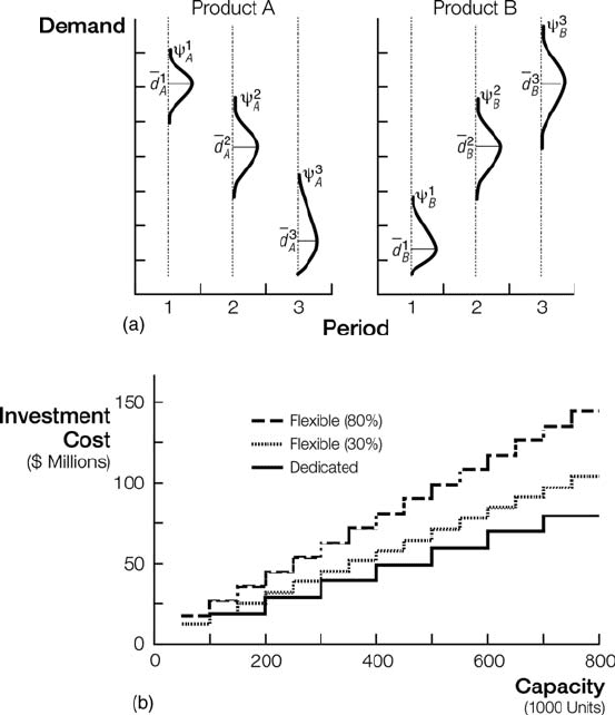
The lower bound for ﬂexible capacity is lower than that of dedicated. Figure 7.2(b)

represents an example cost structure for dedicated and ﬂexible capacity investments,

for ﬂexible premium of 30 and 80%.

Optimization Model: At the beginning of the planning horizon, the ﬁrm ﬁrst

makes a strategic investment decision on the quantity and types of manufacturing

systems to purchase. Once the initial investment decisions are given, the ﬁrm

continually makes tactical, operating decisions every period on how to allocate its

resources in the most proﬁtable way across products.

We need to solve the problem in two stages. First, assuming that a strategic

investment decision is already given, we compute the maximum possible operating

revenue during the entire lifetime of all products (i.e., the planning horizon). Next, we

make the strategic capacity decision by choosing the recommended installed

capacities that will generate the maximum proﬁt that is corresponding to the highest

operating revenue minus investment costs.

Figure 7.2 Example: (a) demand distributions and (b) capacity investments.

182

ECONOMICS OF SYSTEM DESIGN

The problem may be formulated as a linear program with an optimization cost

index R(d,k), which expresses the revenue that can be achieved for a given capacity

investment decision k , and for any fulﬁllment of product demands d over the planning

horizon.

Rðd; kÞ¼max

x;y

t¼1

t1

ðx

þ y

Þþp

ðx

þ y



subject to constraints

ðaÞ x

 k

8t ¼ 1; ...; T

ðbÞ x

 k

8t ¼ 1; ...; T

ðcÞ y

þ y

 k

8t ¼ 1; ...; T

ðdÞ x

þ y

 d

8t ¼ 1; ...; T

ðeÞ x

þ y

 d

8t ¼ 1; ...; T

The decision variables x

and x

denote, respectively, how many units of

dedicated capacity A and B are needed to ﬁll period t demand, whereas the decision

variables y

and y

denote the optimal allocation of the ﬂexible capacity between

products. In addition, b is the discount factor per period that is used to calculate the

NPVof the revenues, b ¼ 1/(1 þ r), where r is the annual rate of return as deﬁned in

Section 7.1. Constraints (a)–(e) guarantee that one will assign neither more capacity

than the maximum available, nor more capacity than demand (i.e., the production

quantities within a period do not exceed available capacity and are bound by the

demand).

Having obtained the maximum operating revenue, we can now write the strategic

decision problem of determining the optimal capacity investments, k.

max

Rðd; kÞðÞc  k

In the above formulation, E

[R(d,k)] is the expected value of the operati ng revenue

where the expectation is taken over demand distributions and ck

represents the total

investment costs. The ﬁrm’s objective is to maximize E

7.2.2 Numerical Examples

We will now solve the above formulated optimization problem for a planning horizon

of three periods. The objective is to explore how investment costs, product revenues,

and demand volatilities affect optimal capacity investment decisions.

Optimal Capacity Investment: In order to analyze the effects of the relative

investment costs on opti mal capacity investment decisions, we ﬁrst consider a base

case constructed by the following problem parameters. Assume demands for products

A and B generate revenues of p

¼ p

¼ 75 and, for a three-period horizon, they have

mean values (600, 350, 100) and (125, 450, 700), and standard deviations (50, 70, 70)

CAPACITY PLANNING STRATEGIES 183

for A and (25, 70, 70) for B. The investment costs for dedicated capacity are

¼ c

¼ 100, and the unit cost for the ﬂexible capacity varies from 100 to 200

corresponding to a ﬂexible premium of 0–100%. To calculate the NPVof the revenues,

we assume a discount factor of b ¼ 0.8.

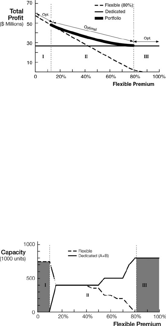
Figure 7.3 shows proﬁts obtained from three different investment strategies: (1)

dedicated capacity only, (2) ﬂexible capacity only, and (3) a portfolio consisting of

both dedicated and ﬂexible systems. The decisi on space has three distinct regions. In

region I—invest in ﬂexible capacity only. In region III, install only dedicated lines. In

region II, however, a portfolio strategy results in strictly higher proﬁts.

Figure 7.4 depicts the quantities of capacity purchases that lead to the optimal

proﬁts shown in Figure 7.3. Speciﬁcally, we observe that as the unit cost for the

ﬂexible capacity increases, a portfolio consisting of gradually increasing share of

dedicated capacities becomes optimal.

Product Revenue: Next, we consider the effects of product revenues on optimal

capacity investments. Figure 7.5 displays the optimal investment decisions for various

product revenues ranging from $30 to $150 per unit. As shown by the ﬁgure, higher

Figure 7.3 Proﬁts obtained by pure ﬂexible, pure dedicated, and portfolio strategies.

Figure 7.4 Optimal capacity investment portfolio.

184

ECONOMICS OF SYSTEM DESIGN

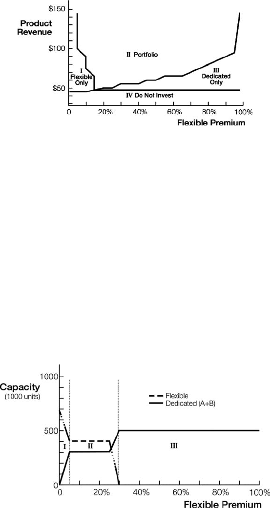
product revenues enlarge the range over which the optimal strategy is of a portfolio

type. The rationale for this interesting conclusion is explained below.

As product revenues get higher, it is more proﬁtable for ﬁrms to increase

production in order to reduce missed demand opportunities. Since dedicated capacity

costs less, it makes sense to build the increased level of total capacity partially by

dedicated systems. On the other hand, employing ﬂexible capacity is also crucial as it

allows allocating capacity when needed and hence enables a higher demand ﬁll rate

and revenues in the presence of demand uncertainties. Therefore a portfolio of ﬂexible

and dedicated systems is optimal over a larger ﬂexible premium range.

Demand Variance: Lastly, we analyze the effect of demand variance on optimal

capacity investment decisions. Figure 7.6 displays the constituents of the optimal

capacity investments when demands exhibit lower volatility. We observe that the

value of the pure ﬂexible investment strategy diminishes (compare to Figure 7.4). In

other words, when market is more predictable, an optimal investment strategy favors

dedicated systems.

Figure 7.5 Effects of product revenues.

Figure 7.6 Effects of demand variance on optimal capacity investment decisions.

CAPACITY PLANNING STRATEGIES 185

7.3 ECONOMICS OF SYSTEM CONFIGURATIONS

The designer of a new manufacturing system should comply a design process that

starts with high-level strategic decisions—which system type is needed: a dedicated, a

ﬂexible-reconﬁgurable, or a portfolio consisting of both. The deliberations on

choosing the right system have been described and analyzed in Sections 7.1 and 7.2.

Forecasting, as mentioned in Section 7.2, provides the required capacity of the

system.

The next step is to calculate the individual operation times that are needed to

produce the part, where the total production time, t, is given. Producing a part may be,

for example, machining a part by a system composed of machining centers and lathes,

or assembling a part by automation or by workers. Machining a part requires the

calculation of the machine optimal cutting speeds (an example is present ed below),

which will affect the total machining time per part, and will eventually affect the

number of machines needed in the system. If the system capacity (which is based on

forecasted demand) and the total time needed to produce a part are given, it is possible

to calcul ate the minimum number of machines or stations needed in the system.

If the daily demand is Q (parts/day), and the total production time per part is t

(minute/part), the minimum number of machin es, N, needed in the system is

calculated by the equation

N ¼

Q  t

Minutes=day available  Machine reliability

ð7:1Þ

When the number N of machines is given, the next step is to decide upon the right

conﬁguration of a system that is composed of N machines. There may be several ways

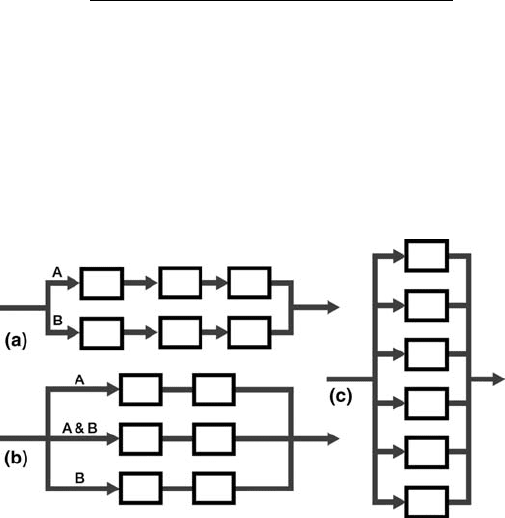
to conﬁgure a multi-stage manufacturing system with a given number of machines.

Figure 7.7, for example, shows three possible conﬁgurations, each with six machines,

and each produces two parts A and B. There are conﬁgurations that require a large

investment in tooling (e.g., Figure 7.7c); in others, a complex material handling

Figure 7.7 Three system conﬁgurations, all with six machines.

186

ECONOMICS OF SYSTEM DESIGN

system increases the investment cost. Note that in the conﬁguration in Figure 7.7a,

each machine performs about one third of the operations neede d to com plete the part,

and therefore the total number of tools in this system is smaller than that in the other

two conﬁgurations.

The selected conﬁguration of the system not only affects the investment cost, but

also has a signiﬁcant impact on the system throughput and on the system respon-

siveness to market changes. Responsiveness includes not only the daily operational

responsiveness of the system to change s in unexpected customers’ orders, but also

convertibility and capacity scalability. All these considerations are part of the system

design process.

There are also operation considerations in selecting a conﬁguration. If the demand

for Part A increases by 33% and at the same day the demand for Part B decreases by

33%, the conﬁguration in Figure 7.7c can supply the new demand (four machines

produce A and two produce B). Satisfying the new demand with the othe r two systems

will not be that simple and will require tool changes during the day, which will reduce

the daily throughput. Therefore, the conﬁguration in Figure 7.7c has the b est

operational responsiveness of these three system s. This system, however, requires

more tools and machines with larger tool magazines, and therefore its capital

investment cost is higher.

7.3.1 Tooling Cost

Let us compare the number of cutting tools needed to place in the tool magazines of

each system conﬁguration in Figure 7.7. Assume that 30 different cutting tools are

needed to produce Part A, and an additional 30 tools (different than those for Part A)

are needed for Part B. In conﬁguration 7.7a, product A is produced by three machines,

and product B is produced by the other three machines. The total number of cutting

tools in system 7.7a is 60 (an average of 10 tools in the tool-magazine of each

machine).

In system 7.7c, if three machines produce part A and three produce part B, then

each machine requires 30 tools (these machines need tool magazines that are three

times larger than the machines in conﬁguration 7.7a) and the total number of tools for

six machines is 180.

In Figure 7.7b, two lines have machines with 15 tools each (namely, 60 tools in four

machines) and two machines in the middle line have 30 tools in each tool magazine

(because they produce both parts A and B). Altogether conﬁguration 7.7b contains

120 tools. Alternatively, if a higher degree of responsiveness is needed, each line must

be able to produce both Part A and B, and then the total number of tools loaded in the

system’s tool magazines is given in Table 7.5.

7.3.2 Impact of Conﬁguration on System Throughput

In the above scenario, from a tooling cost viewpoint, the optimal system is obtained by

conﬁguration 7.7a. However, there are other aspects than just tooling cost assessing

when looking at the operational cost. Let us consider the impact of a single machine

ECONOMICS OF SYSTEM CONFIGURATIONS 187

failure that continues more than a few hours, for example. In systems (a) and (b)

above, the machining sequence is interrupted, and the whole line loses productivity. If

such an event causes the system, or a signiﬁcant portion of it, to shut down, the system

is not adequately responsive. The bottom row of Table 7.5 shows the percentage of

throughput lost when such an event happens. (Note that in Figure 7.7a, 50% is a loss of

the total production; it is 100% for one of the products. Similarly, in Figure 7.7b, 33%

is a loss of the total production; it may be 66% for one of the products.)

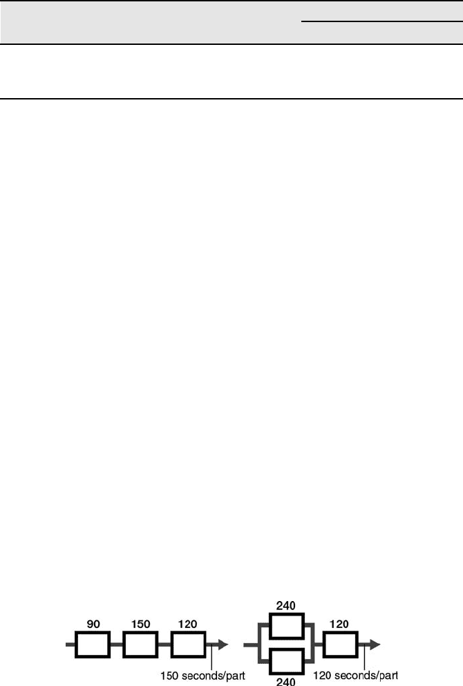
The system throughput is impacted not only by machine failures, but also by the

conﬁguration itself. A simple example that demonstrates the impact of conﬁguration

on throughput is shown in Figure 7.8. To be completed, the part requires three

operations of 90, 150, and 120 seconds. In a serial dedicated line, the slowest

operation (in the second stage) dictates the throughput. The second conﬁguration

has two parallel machines that perform the ﬁrst two operations, and thereby the system

throughput is increased by 25% (150/120).

When selecting a conﬁguration, two measures of responsiveness—system con-

vertibility and scalability—should be considered as well. This issue and others that

inﬂuence the selection of the appropriate conﬁguration are anal yzed in Chapter 10.

7.4 THE ECONOMICS OF BUFFERS

Having buffers to store parts between stations, or machines, in manufacturing systems

is controversial. On one hand, buffers are not value-added-operations, and therefore

adding buffers is a waste according to the Lean principles. However, adding buffers

between unreliable machines increases the system throughput in cases of unpredict-

able events, such as operation time variations, machine failures, and the time required

to repair them. The buffers isolate such disruptive events from propagating in the line.

TABLE 7.5 The Number of Cutting Tools Needed in the Systems Depicted in Figure 7.7

Number of Cutting Tools

7.7a 7.7b 7.7c

System as shown in Figure 7.7 60 120 180

Each machine can produce both Part A and Part B 120 180 360

Loss of throughput if one machine is down 50% 33% 16%

Figure 7.8 Two conﬁgurations with the same number of machines but different

throughputs.

188

ECONOMICS OF SYSTEM DESIGN

Having inﬁnite-size buffers between operations is an extreme case that completely

decouples the operations, such that a failure of a particular machine does not affect the

others in the system. In this case, the slowest machine in the line determines the

system throughput. We will study the issue of a cost-effective buffer size in the case of

serial lines.

The expected throughput of a single isolated machine is proportional to the

machine reliability R that is calculated by

R ¼ MTBF=ðMTBF þ MTTRÞð7:2Þ

where MTBF is the mean time between failures of the machine and MTTR is the mean

time to repair a machine failure. Both machine breakdowns and machine repairs occur

at random.

Serial manufacturing lines may be either synchronous or asynchronous.Ina

synchronous machining line, all machined parts are moving exactly at the same time

from each machine to the next, and all machines start to operate simultaneously. These

lines cannot have buffers between machines. If one machine stops—the entire line

stops.

Building a synchronous machining line is less expensive than building an

asynchronous line, but its reliability is much lower. If the average machine reliability

is R, the line average expected thro ughput is R

of the planned thro ughput of a fully

operational line with n machines. For example, in a line of six machines with an

average machine reliability of R ¼ 0.9, the average expected throughput is only

0.53%.

In asynchronous serial lines, it is not necessarily that all machines start and stop

simultaneously. Machines may stop working because of three reasons: (a) the

machine failed because of a fault or a malfunction; (b) the machine is “starved,”

namely, parts are not available from the upstream buffer or machine (which

apparently stopped to operate); and (c) the machine is “blocked,” namely, it cannot

send the ﬁnished part downstream because the output buffer is full, or (if there is no

buffer) the next machine failed.

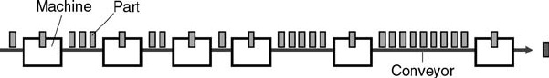
In typical asynchronous serial lines, the machines are connected with a material

transfer device, such as a long conveyor, on which parts may be accumulated (up to a

certain maximum quantity) and wait to be processed on the next machine (see

example in Figure 7.9). This means that between the machines there are buffers that

have maximum part capacity. In other types of asynchronous lines, special buffers are

added between the machines, for example in a form of small closed-loop conveyors,

which also have maximum capacity.

Figure 7.9 Asynchronous serial line with buffer spaces on the conveyor.

THE ECONOMICS OF BUFFERS 189

In asynchronous serial lines without buffers, if one machine fails to opera te, the

entire line does not stop immediately—the upstream and downstream machines

continue to operate until either the failed machine is repaired or the line is purged (all

downstream parts were processed). Asynchronous serial lines with buffers will

continue to operate as long as there are parts in the upstream buffers and empty

spaces in the downstream buffers. Therefore, asynchronous lines have higher

throughput than synchronous serial lines.

The line designer’s dilemma is that adding buffers increases throughput, but

adding buffers create s waste, because it increases the in-process inventory and

contradicts the principles of lean manufacturing. Considering the tradeoff between

throughput gain and inventory increase, buffer space should be limited.

Example: Given an asynchronous serial line with six machines and equal buffers

between machin es. The maximum possible throughput (i.e., production rate witho ut

failures) is 20 parts per hour (cycle time T ¼ 3 minutes). The machines have equal

reliability, with MTBF ¼ 9 minutes and MTTR ¼ 1 minute. Namely, the average

machine reliability, R, is 0.9. The buffers between the machines are equal. What

are the line production rates (in % of the maximum throughput) as function of the

buffer space?

The solution (solved by PAMS software

) is given in the table below:

Buffer size 012345610100

Throughput (%) 71.3 83.7 86.1 87.3 87.9 88.2 88.5 89.1 90

Note that even when the asynchronous line does not have buffers, the throughput is

71%, compared with just 53% of a synchronous line with an average machine

reliability of R ¼ 0.9. The reason is that in the asynchronous line if a machine is down,

the other machines continue to operate and can transfer parts to consecutive operating

machines. The capital investment in a synchronous serial line is lower, but its average

downtime is higher.

A buffer of 1 yields a large marginal increase in the line throughput, and then the

marginal gain becomes smaller as the buffer size increases. If the buffer size is inﬁnite,

every machine is completely decoupled, and the line reliability becomes equal to the

machine reliability. In this example, the line designer wi ll probably add buffers with a

capacity of 4 or 5 parts; the throughput gained with larger buffers than 5 starts to be

marginal.

In the above example, we assumed that the line is balanced, namely, every machine

in the line has an equal operation time. In reality, however, lines are usually not

balanced. In these cases, one of the machines in the line is the slowest, and it is the

bottleneck machine for achieving higher throughput.

Dr. Sam Yang developed the software PAMS at our ERC/RMS. This software utilizes original mathematic

methods (rather than simulation) to calculate the throughput, inventory, and bottlenecks of manufacturing

systems and to optimize their design.

190 ECONOMICS OF SYSTEM DESIGN