Koren B., Vuik K. (Editors) Advanced Computational Methods in Science and Engineering

Подождите немного. Документ загружается.

Yunus Hassen and Barry Koren

Note that the leading order error-term in cell i+ 2 is ﬁrst-order for all

Optimal accuracy in cell i + 2: With (18c) and (19b), we get as semi-discrete

equation for cell i + 2:

i+2

−1

6 −4

i+1

−c

) +

11 −3

i+2

−c

i+1

) +

i+3

−c

i+2

)

= 0. (27a)

Introducing Taylor-series expansions of c

, c

i+1

and c

i+3

around the point i + 2

into (27a), we get as modiﬁed equation for cell i + 2, ignoring the index i + 2:

∂

+ u

∂

−15)

+ (7 −6

)

∂

−24

+ 35)

− (4

−24

+ 19)

∂

= O(h

). (27b)

Equating the leading term of the truncation error to zero, now we get:

7 −6

15 −6

∈





. (28)

This is the value of

that yields the most accurate net ﬂux in cell i + 2. As

opposed to

according to (24), this

is well within the standard

-range

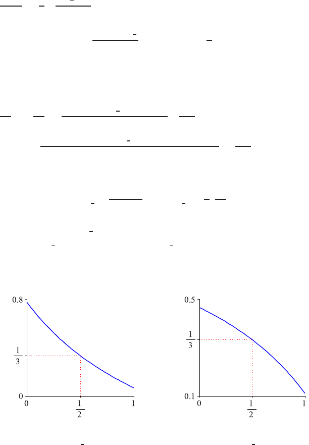
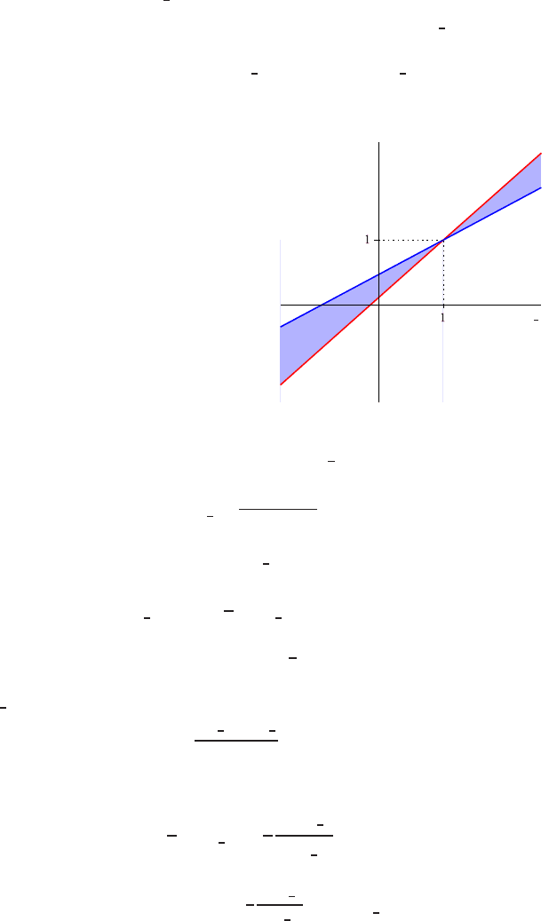
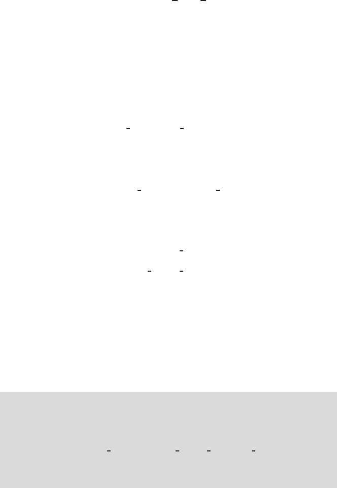
[−1,1]. Its variation for any position of the EB within cell i is depicted in Fig-

ure 7(b).

(a)

i−

(b)

Fig. 7 Variation of the optimal

values for any position of the EB within cell i.

244

Finite-Volume Discretizations and Immersed Boundaries

Substituting the optimal

according to (28) into (27b), we get as modiﬁed

equation for cell i + 2:

∂

+ u

∂

−1

∂

= O(h

). (29)

In contrast to the dispersive error in (25), the dispersive term in (29) does vanish as

the EB gets in the vicinity of the center of cell i,

≈

. We, thereby, get third-order

spatial accuracy, and

according to (28) becomes

(see Figure 7(b), and

the Appendix for a more detailed comparison).

With (17), (18c) and (28), we get as semi-discrete equation for cell i+ 1:

i+1



19 −6

(9 −6

)(5 −2

)

i+1

−c

) +

11 −6

30 −12

i+2

−c

i+1

)



= 0. (30a)

And, substituting Taylor-series expansions for c

, and c

i+2

around the point i + 1,

into (30a), we get as modiﬁed equation for cell i + 1, ignoring the index i + 1:

∂

+ u

∂

−7

∂

= O(h

). (30b)

Equation (30b) shows that we get a ﬁrst-order spatial accuracy in cell i + 1 with a

maximum leading-term truncation-error coefﬁcient of −

uh. Coincidentally, (30b)

is the same as (26b); the leading-order error terms in both equations are identical.

The accuracy loss in the net ﬂux of a neighboring cell is unavoidable. If the cell-face

states were to be ﬁrst-order accurate, i.e. c

= c

and c

= c

i+1

, the modiﬁed

equation for cell i + 1, ignoring the index i+ 1, would become:

∂

3 −2

∂

−

(3 −2

)

∂

= O(h

), (31)

which, for all

, except

, is even zeroth-order accurate.

As the optimal

we choose (28), the one that gives the highest accuracy

in cell i + 2. In summary, the reasons why we choose this

, instead of the one

yielding the highest accuracy in cell i+1 (

according to (24)), are the following:

• For

, we get a third-order (spatial) accuracy in cell i + 2 with (28) (see

(29)). But with (24) we do not get this in cell i+ 1 for any

(see (25)).

The truncation error with (28) is much less than that with (24), for any

(see

Appendix).

• Noting that the solution is discontinuous across an EB, with (28) we have a dis-

sipative leading-error term in cell i+ 1, which is the cell adjacent to cell i (where

the EB is situated), and this makes the solution near the EB less prone to numer-

ical oscillations.

245

Yunus Hassen and Barry Koren

With (24) however, we get the leading-error term in the same cell to be disper-

sive and this makes the solution near the EB to be more susceptible to numerical

oscillations, numerical oscillations which may be hard to suppress because con-

struction of a limiter for cell-face state c

is hard.

• With (28), the accuracy deterioration due to the presence of an EB in cell i is

more conﬁned to the vicinity of the EB. (We get ﬁrst-order (spatial) accuracy

in cell i + 1, and second-order accuracy in cell i + 2; whereas with (24), we get

second-order accuracy in cell i+ 1, and ﬁrst-order accuracy in cell i + 2.)

•

according to (28) is well within the standard

-range [−1,1], but with (24)

we get

∈





3.1.3 Formulae for cell-face states affected by EB

Here, the formulae for all the special cell-face states that are affected by the

EB, in cell i, viz. c

i−

, c

and c

, are summarized.

With (16c) and (21), c

i−

can be rewritten as:

i−

= c

i−1

(3 + 6

)(3 + 2

)

−c

i−1

) +

1 + 6

18 + 12

i−1

−c

i−2

). (32a)

Further, we have:

= c

2 −2

3 −2

i+1

−c

). (32b)

And, with (18c) and (28), c

can be rewritten as:

= c

i+1

11 −6

30 −12

i+2

−c

i+1

) +

(9 −6

)(5 −2

)

i+1

−c

). (32c)

Verify that, in (32a) and (32c), for

, we get exactly the same coefﬁcients

as in the the standard

scheme (see (19a) and (19b)).

246

Finite-Volume Discretizations and Immersed Boundaries

3.2 Spatial monotonicity domains and limiters

Recalling Godunov’s (1959) theorem, all the linear higher-order accurate ﬂuxes,

constructed earlier, may yield wiggles. One negative aspect of wiggles is that they

may cause the solution c to be negative. If c is a physical quantity that should not

become negative (say, density or temperature), this may be highly undesirable. Wig-

gles can be avoided by carefully constraining or ‘limiting’ the advective ﬂuxes cal-

culated by the scheme. By limiting the ﬂuxes, they may become ﬁrst-order accurate

in some solution regions.

A limiter is a nonlinear function that acts like a continuous control between the

higher-order and ﬁrst-order schemes. Obviously, limiters may reduce the overall

accuracy of the scheme to some extent, albeit in non-smooth ﬂow regions only.

Limited schemes are called ‘monotonicity-preserving.’

For the cell-face states that are computed by the standard

scheme (§ 2.3),

the standard

limiter (14b) will be used. In this section, special limiters will be

introduced for the EB-affected cell-face states c

i−

and c

according to formulae

(32a) and (32c). The cell-face state c

, however, will not be limited. This shall be

explained later on.

3.2.1 Spatial monotonicity domain and limiter for cell-face state c

i−

Referring to Figure 6, for cell face i−

, we deﬁne the non-equidistant local succes-

sive solution-gradient ratio ˜r

i−

, as:

˜r

i−

−c

i−1

1+2

i−1

−c

i−2

≡

1 + 2

−c

i−1

−c

i−2

. (33)

Notice that for

, EB in the center of cell i, ˜r

i−

reduces to the standard equidis-

tant solution-gradient ratio known from the theory of standard limiters.

We proceed by rewriting (16c) as:

i−

= c

i−1

(˜r

i−

)(c

i−1

−c

i−2

), (34a)

with

(˜r

i−

) =

1 −

i−

1 +

i−

˜r

i−

. (34b)

Substituting the optimal

i−

according to (21) into (34b), we get:

(˜r

i−

) =

1 + 6

9 + 6

˜r

i−

. (34c)

247

Yunus Hassen and Barry Koren

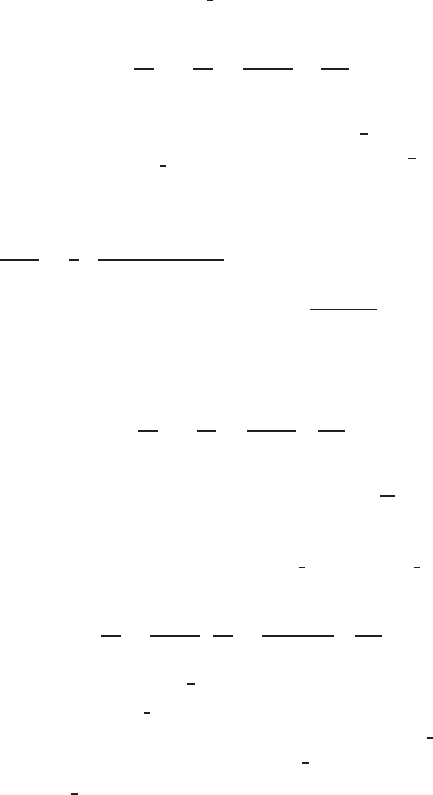
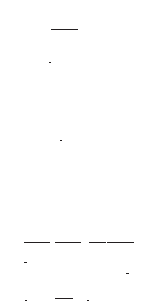
The family of possible

(˜r

i−

) schemes, depending on the position of the EB within

cell i (0 ≤

≤ 1), is represented in Figure 8. The function

(˜r

i−

) will be con-

strained to yield a monotonicity-preserving scheme and to deﬁne the appropriate

limiter for the special cell-face state c

i−

. The argument ˜r

i−

measures the local

monotonicity of the solution.

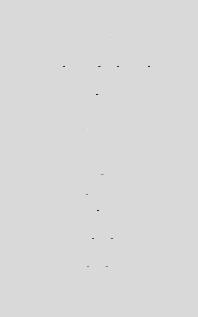
Fig. 8 Family of possible

schemes according to (34c):

the blue line is for

= 1, the

red line is for

= 0, and the

enclosed (colored) region is

for all other

∈ (0,1).

˜r

i−

The local solution-gradient ratio for cell face i−

is deﬁned as:

i−

i−1

−c

i−2

−c

i−3

. (35a)

And, the limited form of cell-face state c

i−

is:

i−

= c

i−2

i−

)(c

i−2

−c

i−3

), (35b)

where

(r) is standard limiter (14b) with

The following monotonicity requirement is enforced, to constrain the function

(˜r

i−

−c

i−

i−1

−c

i−2

≥ 0. (36a)

Substituting (34a) and (35b) into (36a), using (35a), we get as constraint relation:

1 +

(˜r

i−

) −

i−

)

i−

≥ 0. (36b)

The standard limiter already satisﬁes 1−

i−

)

i−

≥0, ∀r

i−

; therefore, the (in)equality

(36b) holds good if:

248

Finite-Volume Discretizations and Immersed Boundaries

(˜r

i−

) ≥ 0, ∀˜r

i−

. (36c)

Moreover, enforcing the additional monotonicity requirement:

−c

i−

−c

i−1

≥ 0, (37a)

and substituting (34a) into (37a), using (34c) and (33), we get:

(˜r

i−

)

˜r

i−

≤ 1 + 2

, ∀˜r

i−

. (37b)

The (in)equalities (36c) and (37b) deﬁne the spatial monotonicity domain for the

special limiter function

(˜r

i−

). They delineate the left and lower bounds of the

domain. The upper bound is still to be derived in § 4 from the fully discrete equa-

tion. Once we also have deﬁned this upper bound, the respective limiter will be

introduced, in § 4.1.

3.2.2 Limiter for cell-face state c

Regarding cell-face state c

, a regular monotonicity argument r

can not be

deﬁned here. A regular monitor uses two solution values upstream of cell faces. In

this case, since we do not want to use solution values from the other side of the EB,

and therefore not c

, we have only one upstream solution, c

, too little to introduce

the regular smoothness monitor. Therefore, c

is not limited.

3.2.3 Spatial monotonicity domain and limiter for cell-face state c

Referring to Figure 6, the monotonicity argument ˜r

is deﬁned, as:

˜r

i+2

−c

i+1

−c

3−2

≡

3 −2

i+2

−c

i+1

−c

. (38)

As expected, for

, ˜r

according to (38) reduces to the known equidistant-

grid ratio. Similar to the rewriting of expression (16c) for c

i−

, here we rewrite

(18c) for c

, as:

= c

i+1

3 −2

(˜r

)(c

i+1

−c

), (39a)

with

249

Yunus Hassen and Barry Koren

(˜r

) =

1 −

1 +

˜r

. (39b)

Substituting the optimal

according to (28) into (39b), we get:

(˜r

) =

15 −6

11 −6

15 −6

˜r

. (39c)

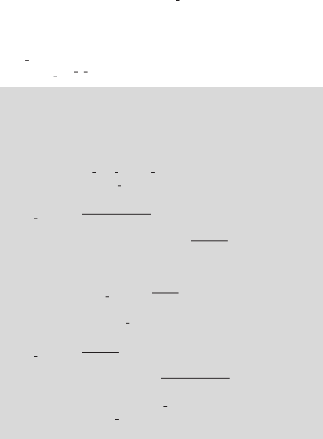
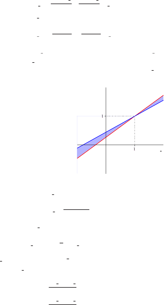
The family of possible

(˜r

) schemes is given in Figure 9. Just as

(˜r

i−

), in

§ 3.2.1, the function

(˜r

) will be constrained to yield a monotonicity-preserving

scheme and to deﬁne the appropriate limiter for the special cell-face state c

Fig. 9 Family of possible

schemes according to (39c):

the blue line is for

= 1, the

red line is for

= 0, and the

enclosed (colored) region is

for all other

∈ (0,1).

˜r

The monotonicity argument r

is deﬁned as:

i+3

−c

i+2

−c

i+1

. (40a)

And, the limited form of c

is:

= c

i+2

)(c

i+2

−c

i+1

), (40b)

where

) is limiter (14b) with

To constrain

), the following monotonicity requirements are enforced:

−c

i+1

−c

≥ 0, (41a)

−c

i+2

−c

i+1

≥ 0. (41b)

250

Finite-Volume Discretizations and Immersed Boundaries

Substituting (17) and (39a) into (41a), we get as restriction for

(˜r

) ≥ −1, ∀˜r

. (42a)

And, substituting (39a) and (40b) into (41b), we get:

(˜r

)

˜r

−

) ≤ 2. (42b)

Since the standard limiter satisﬁes

) ≥ 0, ∀r

, the (in)equality (42b) holds

good if:

(˜r

)

˜r

≤ 2, ∀˜r

. (42c)

The (in)equalities (42a) and (42c) deﬁne the spatial monotonicity domain for the

special limiter function

(˜r

). They delineate the left and lower bounds of the

domain. Once again, after deﬁning the upper bound of the domain in § 4.1, the

respective limiter for the special cell-face state c

will be introduced. Note that

as opposed to the spatial monotonicity domain for c

i−

(see (36c) and (37b)), the

monotonicity domain for c

is independent of

4 Temporal discretization

The semi-discrete equation (4), after substituting the appropriate discretizations for

the spatial operator, is discrete in space but still continuous in time. It can be com-

pactly written as:

= −

−c

i−

) ≡ F(c), (43)

which is an ordinary differential equation that can be discretized in time using a va-

riety of explicit and implicit time integration methods, to get a fully discrete system

of equations. Here, only two explicit schemes are considered: the Forward Euler

method and the three-stage Runge-Kutta, RK3b, scheme [6]. The latter gives third-

order accuracy in time.

For the Forward Euler method, (43) becomes:

n+1

= c

F(c

) ≡ c

−

−c

i−

), (44)

where

= u

/h is the CFL number, and

the time step. Similarly, for the RK3b

scheme, we have:

n+1

= c

+ R

+ 4R

), (45a)

where the R

’s ( j = 1,2,3) are internal vectors that are computed as:

251

Yunus Hassen and Barry Koren

F(c

+ R

), (45b)

F(c

4.1 TVD conditions and time step

The limited numerical ﬂux conditions, as derived in § 3.2, are still insufﬁcient to

guarantee monotonicity during time integration. Harten’s theorem [5] provides ad-

ditional conditions that are necessary for the convergence of the fully discrete so-

lutions to the exact, monotone solutions. These conditions deﬁne the upper bounds

for the limiter functions

(˜r

i−

) and

(˜r

), and consequently result into more

stringent restrictions on the CFL number, than the condition for stability.

The theorem in [5] states that any consistent scheme for a conservation law, writ-

ten in the conservative form:

n+1

= c

− D

−

i−

−c

i−1

) + D

i+1

−c

), (46a)

where the D’s are solution-dependent coefﬁcients, is total-variation diminishing

(TVD) if, for all i:

≥ 0, (46b)

−

+ D

≤ 1. (46c)

The total variation (TV) at time level n is deﬁned, in discrete form, by:

TV(c

) =

∑

i+1

−c

|, (47)

and, any scheme is said to be TVD if TV(c

n+1

) ≤ TV(c

Both conditions, (46b) and (46c), can be interpreted as positive coefﬁcient

requirements. To do so, we rewrite (46a) as

n+1

= D

−

i−

i−1

+ (1 −D

−

i−

−D

+ D

i+1

. (48)

The positive coefﬁcient requirements for (48) are:

252

Finite-Volume Discretizations and Immersed Boundaries

−

i−

≥ 0, (49a)

1 −D

−

i−

−D

≥ 0, (49b)

≥ 0. (49c)

Equation (48) holds for any i, so also for i + 1:

n+1

i+1

= D

−

+ (1 −D

−

−D

i+1

+ D

i+2

. (50)

The positive coefﬁcient requirements applied to (50) yield, among others,

−

≥ 0. (51)

So, with (49c) and (51) we have already interpreted (46b) as a positive coefﬁ-

cient requirement. From (49b) it follows

−

i−

+ D

≤ 1. (52)

Combining (52), (49a) and (49c), it may be written:

0 ≤ D

−

i−

≤ 1 −

, (53a)

0 ≤ D

≤

, (53b)

with

some constant in the range [0,1]. We assume that the upper bound 1−

holds for all i, hence also for D

−

0 ≤ D

−

≤ 1 −

. (54)

Summation of (53b) and (54) gives

0 ≤ D

−

+ D

≤ 1. (55)

Combined with (49c) and (51) this may be reduced to

−

+ D

≤ 1, (56)

which is TVD requirement (46c).

With this we have shown that TVD requirements (46b) and (46c) are

positive coefﬁcient requirements.

253