Koren B., Vuik K. (Editors) Advanced Computational Methods in Science and Engineering

Подождите немного. Документ загружается.

Data Assimilation Algorithms for Numerical Models

state=model.getstate

state=state+delta_state

model.setstate(state)

A disadvantage of this implementation is that it does not provide much ﬂexibility.

The preferred implementation in COSTA is:

model.axpy(1.0,delta_state) //note axpy: y=alpha

x+y

If the model state contains for example concentrations that must be positive at

all time, the model programmer can handle this nicely by implementing the axpy

method. An additional advantage of the axpy-method is that this eliminates the need

for the unnecessary copying of state vectors. When the model interface does not im-

plement the axpy method it will be implemented by COSTA using the getstate and

setstate methods of the model component. In some situation it is not not possible for

COSTA to ﬁll in the missing methods. However this is not always a problem. For

example a model that does not implement an adjoint can still work with the sequen-

tial data assimilation methods in COSTA. It is always possible to add the missing

methods when needed.

COSTA is set up such that it can be used for a wide range of data assimila-

tion and calibration methods. Currently COSTA contains the following sequential

data assimilation methods: Ensemble Kalman Filter (EnKF) (Evensen, 2003), En-

semble Square Root Filter (EnSRF) (Whitaker and Hamill, 2002), Complementary

Orthogonal subspace Filter For Efﬁcient Ensembles (COFFEE) (Heemink et al.,

2001) and RRSQRT Kalman ﬁlter (Verlaan and Heemink, 1997). The model cal-

ibration in COSTA where time independent model parameters are calibrated. The

available methods are: the Conjugate Gradient (CG) method (Fletcher and Reeves,

1964), a Quasi Newton methods using the LBFGS method (Nocedal, 1980 and Byrd

et al.,1994) and the Simplex method (Nelder and Mead, 1965).

5 Applications in coastal sea modeling

5.1 Storm surge prediction using Kalman ﬁltering

Large areas of the Netherlands lie below the mean sea water level, which give rise

to a continuous risk of storm surge ﬂooding. A number of severe ﬂoods of this kind

have occurred in the past. The last disaster in 1953 killed more than 1800 people

and ﬂooded over 340.000 acres of land in the southwest of the Netherlands. In order

to prevent such disaster from recurring, a number of projects concerning safety have

been conducted, which include heightening the dikes and constructing some mov-

able storm surge barriers. In connection to this, accurate storm surge predictions

at least six hours ahead, are necessary to decide what precautionary actions have

to be taken to protect the dikes and for proper closure of the movable storm surge

barriers. Since the mid-1980s, these predictions are based on a numerical hydrody-

123

A.W. Heemink et al.

namic model called the Dutch Continental Shelf Model (DCSM). To increase the

predictive capability, in the operational system observed water level is assimilated

to the DCSM. In this section we describe the DCSM and data assimilation technique

applied to it, which is used operationally in the Netherlands.

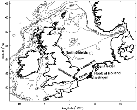
The DCSM covers the area of the north-east European continental shelf, i.e.

W to 13

E and 48

N to 62

N as shown in Figure 3. It is based on the two

dimensional non-linear shallow water equations, which describe the large-scale mo-

tion of water level and depth-integrated horizontal ﬂow. (Gerritsen, et.al. [1995]).

At closed boundaries (coastlines) the ﬂow velocity perpendicular to the coastline is

set to zero. On the other hand, at open boundaries, the ﬂow velocity parallel to the

boundaries is set to zero and tidal harmonic water set-up is speciﬁed with ten tidal

constituents: M2, S2, N2, K2, O1, K1, Q1, P1, NU2, and L2.

Fig. 3 DCSM area with some water-level observation stations used in assimilation

To solve the system of equations which describes the model, discretization using

an Alternating Directions Implicit (ADI) method and a staggered C-grid is used. The

numerical scheme is developed by Stelling (1984) based on the work of Leendertse

(1967), solved in spherical grid (e.g. Verboom, et.al. [1992]). The resolution of the

spherical grid is 1/8

×1/12

, which is approximately 8 ×8 km. This conﬁguration

results in 201 ×173 computational grid cells with 19809 active cells. The time step

is 10 minutes. This model uses forecasts of the KNMI (Netherlands Meteorological

Institute) meteorological high-resolution limited area model (HiRLAM) as input.

Since 1992, a special feature of DCSM has been added, which is the use of as-

similation of real-time measurements from tide gauges using a steady-state Kalman

ﬁlter (Heemink and Kloosterhuis, 1990). The objective of the implementation of this

ﬁlter is to improve the initial state from which to start the forecast. This ﬁlter assim-

124

Data Assimilation Algorithms for Numerical Models

ilates the selected water level observations from eight tide gauges at the British and

Dutch coasts (see Figure 3). Observations from British gauges during the period of

surge coming from the Atlantic, contain information on the surge in the Southern

North Sea several hours ahead. If they can be assimilated into the model, external

surges can be included and errors due to imperfect meteorology during this period

can be corrected for (Gerritsen et.al., 1995).

The implementation of the Kalman ﬁlter requires a conceptual change from the

deterministic model into a stochastic model. This is done by adding error terms

to the deterministic model. In the operational DCSM, the errors in the model are

assumed to be introduced by the uncertainty in the wind input. In the operational

system, this uncertainty is accounted for by adding error terms to the u and v depth-

average velocities (Heemink and Kloosterhuis, 1990).

The implementation of the Kalman ﬁlter on the DCSM is done by exploiting the

fact that the observations come from a ﬁxed network and by assuming that the er-

ror statistics in the model and the observations vary only slightly in time (Gerritsen

et.al., 1995). This means that the solution for the covariance equations in Section

3.2 will become constant after several recursions. Since the propagation of the er-

ror covariance is independent from the real observation, it is possible to compute

the steady-state Kalman gain off-line. The use of the steady-state Kalman ﬁlter has

the advantage of being computationally cheap. It leads to only 10% extra computa-

tional cost (Gerritsen et.al., 1995). For the operational system, the computation of

the steady-state Kalman gain is carried out by using a Chandrasekhar-type algorithm

(Heemink and Kloosterhuis, 1990). Another ensemble type algorithm for comput-

ing the steady-state Kalman gain implemented on DCSM is proposed by Sumihar,

et.al [2008]. Once the Kalman gain is computed, the original non-linear model is

used to propagate the mean for prediction.

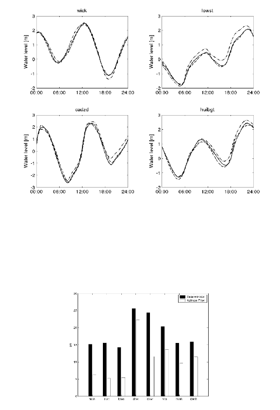
To illustrate the effect of implementing steady-state Kalman ﬁlter on DCSM,

in Figure 4 we show the time series of water level on the whole day of 12 Jan-

uary 2005, obtained from observation, model results with and without assimilation

at four locations. Two of these stations (Wick and Lowestoft) are located on the

British coast, of which the data is used for assimilation. On the other hand, the other

two stations, Cadzand and Huibertgat, are located in the South-west and North of

the Netherlands respectively. The data from the latter are not used for the assimi-

lation. By visual check on Figure 4, we see that by assimilation, the model results

are pulled closer towards the observation. To acquire a better idea about the ﬁlter

performance in assimilating observed data, the root-mean-square (RMS) of water

level innovation is computed over the simulation period of 1 November 2004 - 1

February 2005. The RMS innovation of water level is computed both for assimila-

tion and validation stations. Assimilation station is the station whose data is used

for assimilation, while validation station is the one where data is used for validation

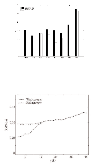
but not for assimilation. The results are presented in Figures 5-6. It is clear from

these pictures that the Kalman ﬁlter reduces the RMS innovation of water level in

both assimilation and validation stations. This indicates that the correction is prop-

agated spatially consistent as it also applies to locations where data is not used for

assimilation. This demonstrates that the ﬁlter succeeds in forcing the model closer

125

A.W. Heemink et al.

to the observation. The steady-state Kalman ﬁlter is used in operational system for

reinitializing the model before making forecast. The output is evaluated every few

months, after every severe storm and if the hydrologist or meteorologist indicates

any ﬂaws. To illustrate the forecast performance, we show in Figure 7 an example of

operational validation, consisting the RMS forecast errors with and without Kalman

ﬁlter (Verlaan, et.al. 2005).

Fig. 4 Water level time series at Wick, Lowestoft, Cadzand, and Huibertgat on 12 January 2005.

The dashed lines represent observed water level, the dash-dotted lines model results without as-

similation, and the full-lines model results with assimilation.

Fig. 5 RMS innovation of water level at assimilation stations

126

Data Assimilation Algorithms for Numerical Models

Fig. 6 RMS innovation of water level at validation stations

Fig. 7 Operational evaluation for location Scheveningen. RMS errors for different forecast ranges

with and without Kalman ﬁlter (picture is taken from Verlaan, et.al [2005])

5.2 Using an RRSQRT Kalman ﬁlter to assimilate HF radar data

into a 3D coastal ocean model

5.2.1 Introduction

This section presents extensive experiments that have been done with a time-

dependent Kalman ﬁlter for a large-scale, three dimensional numerical model of

the coastal region near IJmuiden in the Netherlands (the IJmond model). The ﬁl-

ter has been used to assimilate high frequency(HF)-radar measurements and ADCP

127

A.W. Heemink et al.

measurements into the model. The experiments have been done both to show that

Kalman ﬁltering for such large-scale models is feasible and to investigate the 3D ef-

fects in the data-assimilation. The IJmond region is the region around IJmuiden, on

the North-West coast of the Netherlands. It is the entrance to the Noordzee channel,

which leads to the port of Amsterdam, the capital of the Netherlands. Apart from

this, the IJmond region is economically important in its own right.

In regions like IJmond, 3D models are far superior to 2D models because they

are capable of representing stratiﬁcation and the related ﬂow phenomena. A proper

representation of these phenomena is needed to bring in large ships under strong

ﬂow conditions. Without such models, large ships have less opportunities to safely

enter the harbor or the Noordzee channel, which has an obvious negative economic

effect.

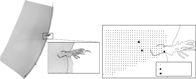
HF radar velocity

ADCP velocity

waterlevel

Fig. 8 Left: The computational grid for the IJmond model.

Right: Locations of the observation points.

The region of interest covers some 70 km along the coast and stretches some 40

km into the sea (see Figure 8). It is a rather shallow, sandy region with a maximum

depth of about 28 meters. The main feature is a channel in the bottom to allow

taller ships to enter the harbor, and a very deep pit just before the entrance to the

harbor. The ﬂow is predominantly along-shore. The entrance to the harbor itself is

protected by two piers, one to the north and one to the south. The harbor is known for

signiﬁcant short-term variations in water level within the harbor. Sweet water enters

the region from the Noordzee channel at moments when the sluices are opened. This

means that there is a very relevant interaction between sweet and salt water in the

IJmond region.

5.2.2 The TRIWAQ model for the IJmond region

The numerical model used for this study is the 3D ﬂow model TRIWAQ. It is the

3D variant of the WAQUA model, which is an operational software system used

128

Data Assimilation Algorithms for Numerical Models

for a wide range of applications by the Directorate for Public Works and Water

Management. This directorate is responsible for the management of the major water

systems in the Netherlands, including the coastal region.

−16 −14 −12 −10 −8 −6 −4 −2 0 2

0.05

0.1

0.15

0.2

0.25

0.3

0.35

0.4

z−location [m−NAP]

stddev amp [m]

ADCP−A (04−Dec−1998 00:00:00)−(05−Dec−1998 09:45:00)

No filtering

ADCP−A

−16 −14 −12 −10 −8 −6 −4 −2 0 2

0.5

1.5

z−location [m−NAP]

stddev dir [rad]

ADCP−A (04−Dec−1998 00:00:00)−(05−Dec−1998 09:45:00)

No filtering

ADCP−A

−16 −14 −12 −10 −8 −6 −4 −2 0 2

0.05

0.1

0.15

0.2

0.25

0.3

0.35

0.4

z−location [m−NAP]

stddev amp [m]

ADCP−B (04−Dec−1998 00:00:00)−(05−Dec−1998 09:45:00)

No filtering

ADCP−A

−16 −14 −12 −10 −8 −6 −4 −2 0 2

0.5

1.5

z−location [m−NAP]

stddev dir [rad]

ADCP−B (04−Dec−1998 00:00:00)−(05−Dec−1998 09:45:00)

No filtering

ADCP−A

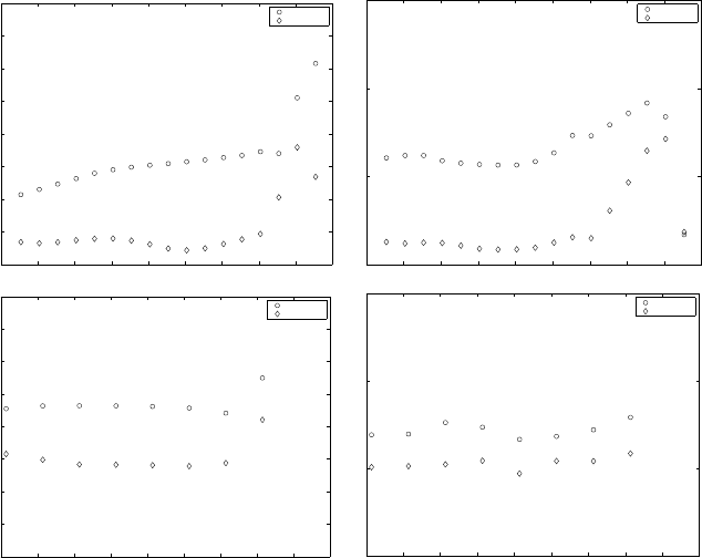
Fig. 9 Standard deviation of the difference between observed and predicted velocity in ADCP-

point A (top) and ADCP-point B (bottom) with and without assimilation of actual data from ADCP

A. The left-hand plots apply to the magnitude of the velocity, the right-hand plots apply to the

direction.

TRIWAQ is based on a ﬁnite-difference discretization of the shallow water equa-

tions and includes a transport model for salinity and temperature. Forcing is done

by boundary conditions which can be composed of different combinations of water

level, ﬂow velocity and discharge. The wind can be applied uniformly or through

a spatially varying wind velocity and pressure. Bottom-friction is modeled through

ezy coefﬁcients computed according to the Manning or the White-Colebrook

equations. TRIWAQ has extensive features for the modeling of drying and ﬂooding

and for special hydrodynamic objects such as barriers, weirs and sluices.

The IJmond region is modeled in TRIWAQ by a curvilinear grid with a maximum

extension of 188 grid-points along the coast and 230 grid-points in the cross-shore

direction (see Figure 8). The grid is highly contracted around the harbor area to

give a high resolution there. In vertical direction, the ﬂow ﬁeld is modeled with four

equidistant sigma layers. This is much less than what is common for coastal models

129

A.W. Heemink et al.

(which usually apply more than ten layers). The main reason for using such a small

number of layers is to keep the amount of computations within limits. At the same

time, it should be able to represent at least some of the vertical dynamics. The time

step is half a minute, mainly to accommodate for the ﬁne mesh inside the harbor.

Boundary conditions are given along the sea-perimeter of the model. The boundary

conditions are determined from a 2D model of the entire Dutch coastline.

−16 −14 −12 −10 −8 −6 −4 −2 0 2

0.05

0.1

0.15

0.2

0.25

0.3

0.35

0.4

z−location [m−NAP]

stddev amp [m]

ADCP−A (04−Dec−1998 00:00:00)−(04−Dec−1998 18:50:00)

No filtering

All

selected HFR

ADCP−A

−16 −14 −12 −10 −8 −6 −4 −2 0 2

0.5

1.5

z−location [m−NAP]

stddev dir [rad]

ADCP−A (04−Dec−1998 00:00:00)−(04−Dec−1998 18:50:00)

No filtering

All

selected HFR

ADCP−A

−16 −14 −12 −10 −8 −6 −4 −2 0 2

0.05

0.1

0.15

0.2

0.25

0.3

0.35

0.4

z−location [m−NAP]

stddev amp [m]

ADCP−B (04−Dec−1998 00:00:00)−(04−Dec−1998 18:50:00)

No filtering

All

selected HFR

ADCP−A

−16 −14 −12 −10 −8 −6 −4 −2 0 2

0.5

1.5

z−location [m−NAP]

stddev dir [rad]

ADCP−B (04−Dec−1998 00:00:00)−(04−Dec−1998 18:50:00)

No filtering

All

selected HFR

ADCP−A

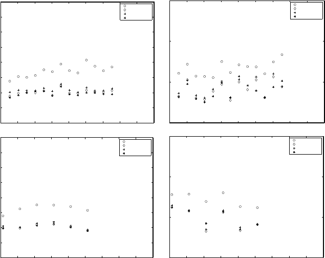
Fig. 10 Standard deviation of the difference between observed and predicted velocity in ADCP-

point A (top) and ADCP-point B (bottom) with and without assimilation of different kinds of

artiﬁcial data. The left-hand plots apply to the magnitude of the velocity, the right-hand plots apply

to the direction.

5.2.3 Kalman ﬁltering for large 3D models

The quality of model predictions can be improved by applying data-assimilation:

using observations of the actual ﬂow situation to correct the model state so that the

ensuing predictions are better. One of the methods to perform data-assimilation is

Kalman ﬁltering.

The full Kalman covariance matrix in the case of the IJmond model would be

about 700.000×700.000 elements. The RRSQRT algorithm reduces this to a ma-

130

Data Assimilation Algorithms for Numerical Models

trix of 700.000×50 elements. Even with the RRSQRT approximation, computing

requirements are still excessive. But they can be handled on large scale parallel

computing facilities. Computing facilities that employ some form of parallelism are

quickly becoming a commodity. Modern PC’s use almost exclusively multi-core

processors and the use of computing-clusters is far from exceptional. In order to

use this type of hardware, a parallel version has been developed of the RRSQRT

Kalman ﬁlter implementation that is available for TRIWAQ. This parallel version

shows excellent speedup ﬁgures on up to 32 processors.

To show the feasibility of data-assimilation for a large scale 3D model, experi-

ments have been done using data from an extensive observation campaign that has

been done in 1998. This campaign involved the already existing tide gauge at one of

the harbor piers, two ADCP moorings just outside the harbor and an HF radar system

(see Figure 8). The ADCP’s are 1200 kHz workhorse ADCP’s, providing velocity

data for bins of 1 meter (Point A) and 2 meters (Point B). ADCP A is located just

outside the south pier, ADCP B is located somewhat further to the north-west. The

HF radar system has been located at the Harbor Operation Center (HOC) next to the

harbor and at Bloemendaal aan Zee, some ﬁve kilometers to the south. It has pro-

vided observations on a grid of 250×250 meters. There are about 450 grid points,

covering an area of about 7 ×4 km.

−0.1

−0.08

−0.06

−0.04

−0.02

0.02

0.04

0.06

0.08

0.1

92 93 94 95 96 97 98 99 100 101 102

495

496

497

498

499

500

RDX [km]

RDY [km]

mean adc u

−0.1

−0.08

−0.06

−0.04

−0.02

0.02

0.04

0.06

0.08

0.1

92 93 94 95 96 97 98 99 100 101 102

495

496

497

498

499

500

RDX [km]

RDY [km]

stdd adc u

−0.1

−0.08

−0.06

−0.04

−0.02

0.02

0.04

0.06

0.08

0.1

92 93 94 95 96 97 98 99 100 101 102

495

496

497

498

499

500

RDX [km]

RDY [km]

mean adc v

−0.1

−0.08

−0.06

−0.04

−0.02

0.02

0.04

0.06

0.08

0.1

92 93 94 95 96 97 98 99 100 101 102

495

496

497

498

499

500

RDX [km]

RDY [km]

stdd adc v

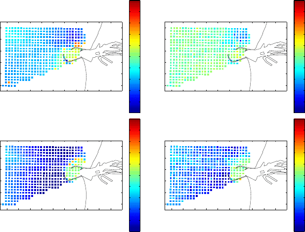
Fig. 11 Effect of assimilation of artiﬁcial data from ADCP A on the mean and standard-deviation

of the difference between predicted and observed velocities in HF-radar points. Colors mark values

in [ms

−1

]. Red colors indicate a deterioration, blue colors an improvement.

131

A.W. Heemink et al.

5.2.4 Results

The data-assimilation scheme itself works properly. Assimilating observations from

only ADCP A gives improvements also at the location of ADCP B some distance

away (see Figure 9). This illustrates that the adaptations made by the ﬁlter have

physical meaning. But the errors in HF-radar points do not beneﬁt from the adap-

tations. This is most likely to be attributed to the poor quality of the HF-radar data

itself. Analysis of this data has shown that it often displays rather erratic ﬂow pat-

terns. Even during the observation campaign, there were doubts about the quality

of the observations. Hence, any deﬁnite conclusions with respect to the HF-radar

data can not be drawn from these experiments. To determine whether better-quality

HF-radar observations could be beneﬁcial, an experiment has been done in which

artiﬁcial HF-radar observations have been assimilated. The artiﬁcial observations

have been obtained from a run of the IJmond model with modiﬁed forcings. The

modiﬁcations to the forcings have been made in such a way that they match the

assumptions of the ﬁlter about the errors in the model. In this way, when the model

is run with the original, unmodiﬁed forcings, the ﬁlter should be able to reconstruct

the state from the distorted model by assimilating the artiﬁcial observations.

The experiments with artiﬁcial data show more consistent results than those using

the actual observations. In this case, the errors in the predictions at HF-radar obser-

vation locations are reduced by the assimilation of ADCP observations (see Figure

11). Furthermore, Figure 10 shows that assimilation of a selection of HF-radar ob-

servations also improves the predictions below the sea-level. The improvements are

comparable to those obtained by assimilating the ADCP observations. So, under cer-

tain assumptions it is possible to reconstruct a 3D ﬂow pattern based on 2D HF-radar

observations. But the experiment is highly idealized. The uncertainty model used to

distort the forcings exactly matches the uncertainty model assumed by the Kalman

ﬁlter, which is usually not the case. Also, the HF-radar observations are assumed

to have independent and small observation errors. In particular the assumption of

independent errors is probably not correct in real HF-radar systems.

In conclusion, the experiment has primarily shown that data-assimilation based

on RRSQRT Kalman ﬁltering for large-scale 3D coastal ocean models is feasible

with current technology.

6 Applications in atmospheric chemistry modeling

Elevated concentrations of ozone in the boundary layer (ﬁrst 3 km of the atmo-

sphere) can cause adverse affects to humans and ecosystems (EC, 2002). Ozone

in the boundary layer is formed by chemical reactions of the ozone precursors, ni-

trogen oxides (NO

), volatile organic compounds (VOCs), and carbon monoxide

and methane under the inﬂuence of sunlight. The impact of ozone is not limited

to the area close to where the ozone precursors are emitted. Transboundary ﬂuxes

transport these precursors over distances of hundreds of kilometers (Lelieveld et al.,

132