Knapp J.S., Cabrera W.L. Metabolomics: Metabolites, Metabonomics, and Analytical Technologies

Подождите немного. Документ загружается.

Correlations - and Distances - Based Approaches to Static Analysis… 67

The three approaches based on the three kinds of distance are: Andrews curves (Andrews,

1972; Barnett, 1976; Everitt and Dunn, 1992), correspondence analysis (CA) (Greenacre,

1984, 1993; Mortier and Bar-Hen, 2004) and Jackknifed Mahalanobis distance (Swaroop and

Winter, 1971; Robinson, 2005), respectively. These different methods provide

complementary diagnostics of the states of individuals in a dataset, leading to extract a

diversity of outliers under different criteria: among all the extracted outliers, the most marked

can be identified as points confirmed by the three diagnostics (Semmar et al., 2008).

Another approach used in multivariate data, consists in performing multiple regression

analysis between a depend variable Y and several explanative ones X

, then a scatter plot can

be visualized between observed and predicted Y (Y

obs

vs Y

pred

) (Figure 54). However, this

approach has the disadvantage to be model-dependent by opposition to the three distance-

based approaches which advantageously extract independent-model outliers.

V.6.1. Standard Mahalanobis Distance Computation

This section presents the basic concepts of the Mahalanobis distance (MD) computation;

it will be followed by a presentation (

V.6.2) of the Jackknifed technique which is mainly used

to calculate robust MD. The two techniques (ordinary and Jackknifed) will be illustrated by a

numerical example.

The Mahalanobis distance provides a multivariate measure of how much a multivariate

point is far from the centroid (average vector) of the whole database. Using Mahalanobis

distance, we can assess how similar/dissimilar each profile x

is to a typical (average)

profile

x .

The Mahalanobis distance takes into account the correlation structure of the data, and it is

independent of the scales of the descriptor variables. It is computed as (Rousseeuw and

Leroy, 1987):

iii

xxCxxMD )()(

−−=

−

, (eq. 1)

Where:

is the squared Mahalanobis distance of the subject i from the average vector (or

centroid)

),...,(

1 p

xxx ,

: a p-row vector (x

, x

,…,x

) representing subject i (e.g. patient i) characterized by p

variables (e.g.

p concentration values measured at p successive times).

x : vector of the arithmetic means of the p variables

∑

(with n : total number of individuals) (eq. 2)

C: the covariance matrix of the p variables

∑

−−

−

xxxx

)()(

(eq. 3)

Nabil Semmar 68

The Mahalanobis distance measures how far is each profile x

from the average profile x

in the metric defined by C. It is the Euclidean distance if the covariance matrix is replaced by

the identity matrix. The purpose of these MD

² is to detect observations for which the

explanatory part lies far from that of the bulk of the data: according to Mahalanobis criteria, a

subject i described by p variables j tends to be outlier if its coordinates x

increase the

variance of the variable j by comparison with all other coordinates x

(k≠i). This situation can

be due to:

- a great difference of x

to the mean

x (high numerator) (eq. 1).

- a weak variance s

² of the variable j, i.e. when the set of values x

(k≠i) represents a

homogenous group (weak denominator) (eq. 1).

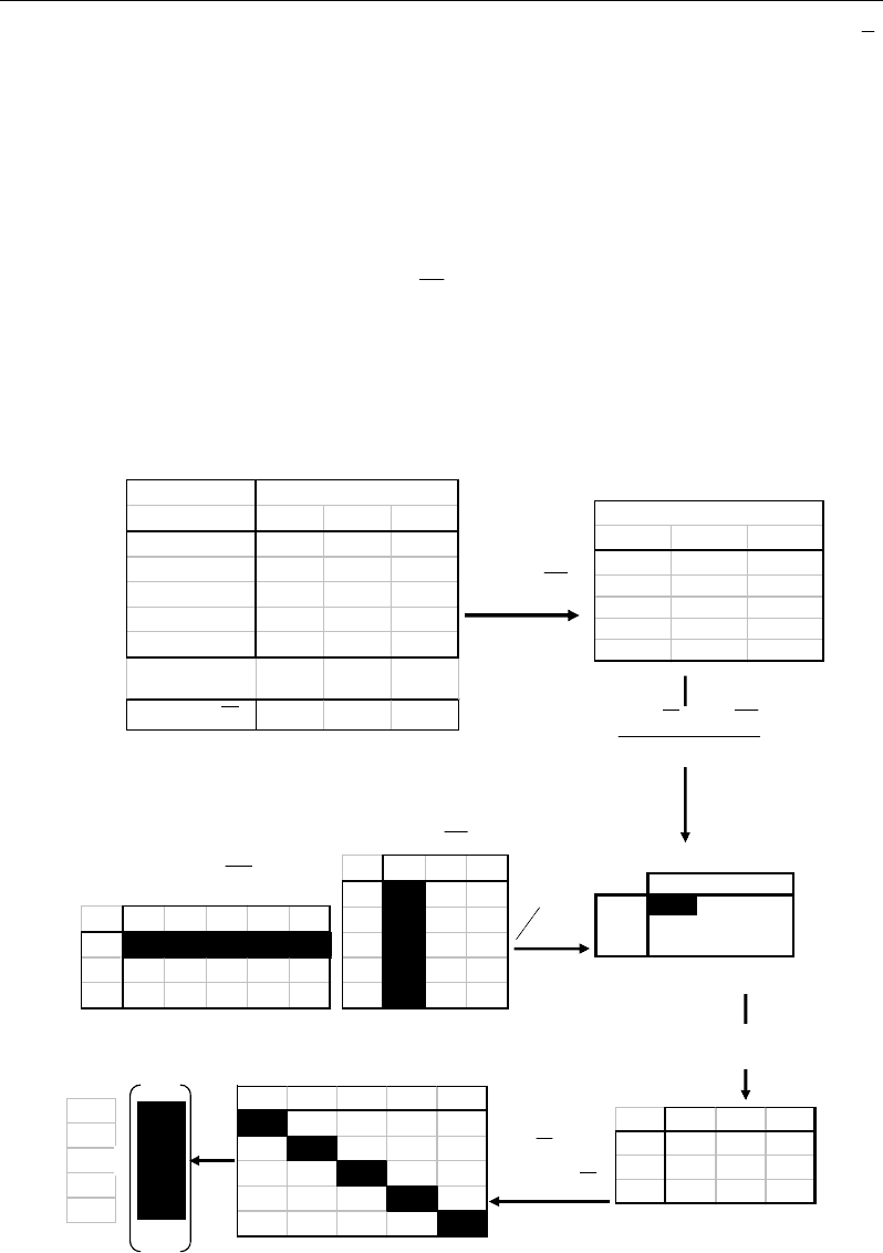
Let’s illustrate the Mahalanobis calculus by a numerical example (Figure 55):

X1 X2 X3 X4 X5

-0.6 -0.6 0.4 2.4 -1.6

M2 -1.2 -1.2 -2.2 0.8 3.8

M3 14.2 -3.8 -2.8 -1.8 -5.8

M1 M2 M3

X1 -0.6

-1.2 14.2

X2 -0.6

-1.2 3.8

X3 0.4

-2.2 -2.8

X4 2.4

0.8 -1.8

X5 -1.6

3.8 -5.8

X =

−

i = 1 to n =5 j = 1 to p=3 metabolites

individuals

M1 M2 M3

1220

122

213

444

070

Average

1.6 3.2 5.8

)()'(

−

−−

XXXX

j = 1 to p=3 metabolites

M1 M2 M3

-0.6 -1.2 14.2

-0.6 -1.2 -3.8

0.4 -2.2 -2.8

2.4 0.8 -1.8

-1.6 3.8 -5.8

XX )( −

)( XX −

C = Variance-Covariance

matrix

()

1−n

-1

M1 M2 M3

0.48 0.1 0.02

0.1 0.23 0.03

0.02 0.03 0.02

XX )( −

X1 X2 X3 X4 X5

3.2

-0.79 -0.81 -0.8 -0.8

-0.79

1.21

1.07 -1.24 -0.25

-0.81 1.07

1.44

-0.39 -1.32

-0.8 -1.24 -0.39

3.1

-0.68

-0.8 -0.25 -1.32 -0.68

3.05

Squared Mahalanobis

distances (in diagonal)

Inverse of Var-Cov matrix

Mahalanobis

distances

1.79

1.10

1.20

1.76

1.75

)(

−

− CXX

M1 M2 M3

M1 2.3

-0.9 -0.6

-0.9 5.7 -7.45

M3 -0.6 -7.45 65.2

√

Figure 55. Numerical example illustrating the calculus of multivariate Mahalanobis distance.

Correlations - and Distances - Based Approaches to Static Analysis… 69

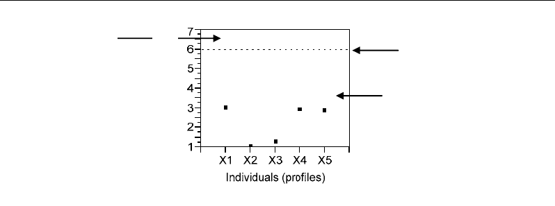
Cut-off value = 5.99

= χ²(df=2, α=0.05)

Non-outlier area

Squared Mahalanobis

distance (MD

)

Outlier area

Figure 56. Graphical representation of the Mahalanobis distance by reference to a Chi-2 cut-off value

with (p-1) degree of freedom.

The MD

values follow a chi-squared distribution with (p-1) degrees of freedom (Hawkins, 1980). The

multivariate outliers can be identified as points having Mahalanobis distances higher than the cut-off

value with a given alpha-risk (e.g. α≤0.05) (Figure 56). Moreover, the most identical profiles to the

centroid are those which have the least Mahalanobis distances; therefore they can be considered as the

most representative of the population (Figure 56, X2, X3 points). In our simple example, the number p

of variables is equal to 3, and the freedom df is equal to p-1=2. For a α risk fixed to 5% (α=0.05), the

cut-off χ² value corresponding to df=2 is given by χ²(2, 0.05)=5.99. From the numerical example, no

squared Mahalanobis distance is higher than this cut-off value; consequently, we conclude that there are

not outliers at the threshold α=5%.

This first part illustrated how Mahalanobis distance is calculated and interpreted in order

to detect outliers. However, the standard Mahalanobis distance suffers from the fact that it is

very sensitive to the presence of outliers in the sense that extreme observations (or groups of

observations) departing from the main data structure can have a great influence on this

distance measure (Rousseeuw and Van Zomeren, 1990). This is somewhat unclear because

the Mahalanobis distance should be able to detect outliers, but the same outliers can heavily

affect the Mahalanobis distance; the reason is the sensitivity of arithmetic mean and

covariance matrix to outliers (Hampel et al., 1986): the individual X

contributes to the

calculation of the mean, and this mean will be then subtracted from X

to calculate its

Mahalanobis distance. Consequently, the standard Mahalanobis distance MD

can be biased,

the outlier X

can be masked and other points can appear more outlying than they really are.

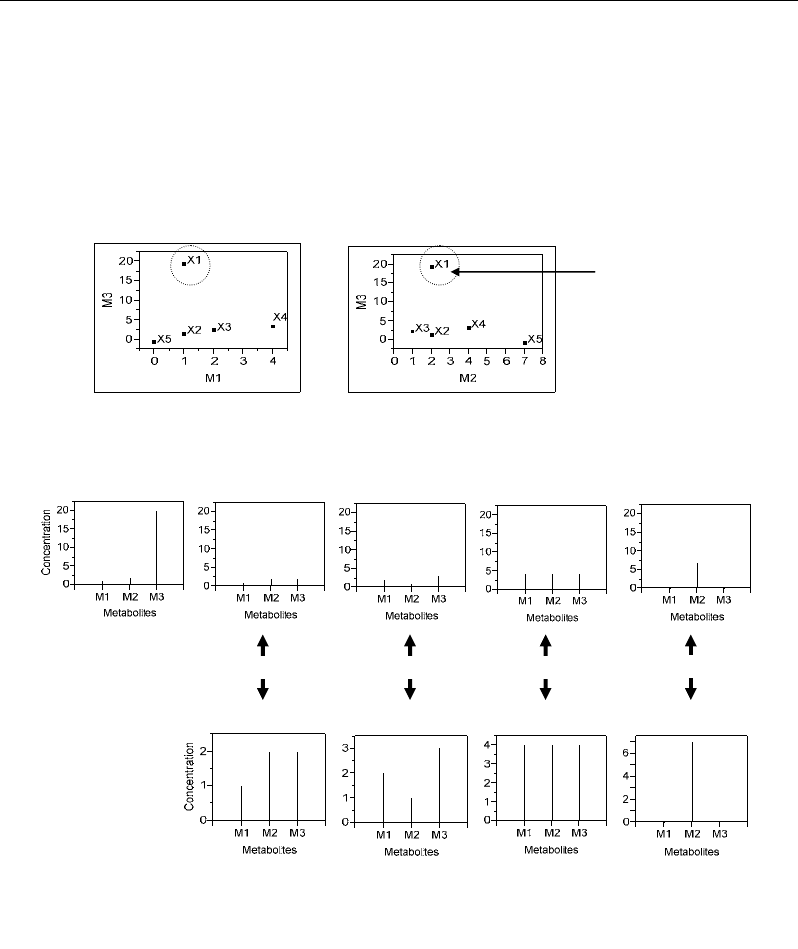
This can be illustrated by the individual X1 which has an atypically high value for the

variable M3 (M3=20) (Figure 57b), but which was not detected as outlier in spite of its higher

MD value (Figure 57a). Moreover, scatter plots of variables M3 vs M1 and M2 showed that

individual X1 corresponds to a relationship outlier analogous to that of point c in Figure 54.

A solution consists in inserting more robust mean and covariance estimators in equation

(1): the Mahalanobis distance can be alternatively calculated by using the Jackknife

technique.

V.6.2. Jackknifed Mahalanobis Distance Computation

Jackknife technique consists in computing, for each multivariate observation x

, the

distance MD

from a mean vector and a covariance matrix which were estimated without the

Nabil Semmar 70

observation x

. This avoids the mean and covariance to be influenced by the values of the

subject i. In fact, a subject i with a high value can be more easily detected as far from the

centroid if it did not contribute to the calculation of mean. Consequently, any multivariate

observation x

characterized by an atypical value x

can be more easily detected as far from

the centroid and/or as discordant by reference to the multivariate distribution of the whole

dataset X (Figure 58).

Relationship

outlier

(a)

X2 X3

X4 X5

X2 X3

X4 X5

Zoom Zoom Zoom

Zoom

(b)

(c)

Figure 57. (a) Scatter plots between different variables showing a relationship-outlier because of

atypically high coordinate for one variable M3 and ordinary coordinates for the other variables M1,

M2. (b, c) Concentration profiles of the five analysed individuals X1-X5 characterized by three

metabolites M1-M3.

The powerful of Jackknife technique can be illustrated by its ability to detect individual

X1 as outlier because of its extreme value for the variable M3 resulting in a distorted profile

compared to the four other profiles (Figure 57b). Moreover, individuals X4 and X5 were

detected as outliers although their values had comparable levels to those of most of the

profiles (Figure 57b). The fact that X4 and X5 are detected as outliers is not due to the levels

of their values but to atypical combinations of the three values (M1, M2, M3) resulting in

atypical profiles (Figure 57c): X4 had uniform profile because of equal values for the three

variables, whereas X5 showed a single needle profile because of the null values of the

variable M1 and M3.

Correlations - and Distances - Based Approaches to Static Analysis… 71

Outliers

Zoom

Squared Jackknife

Mahalanobis distance

Squared Jackknife

Mahalanobis distance

■ ■

■

Figure 58. Outlier detection based on Mahalanobis distance calculated by the Jackknife technique. MD:

Mahalanobis distance.

V.6.3. Outlier Screening from Correspondence Analysis

V.6.3.1. General Concepts of Correspondence Analysis

Correspondence analysis (CA) is a multivariate method that can be applied on a data

matrix having both additive rows and columns, in order to analyze the strongest associations

between individuals (rows) (e.g. patients) and variables (columns) (e.g. metabolites). On this

basis, individuals strongly associated with some variables can be characterized by original or

atypical profiles compared to the whole population. A strong association between an

individual and a variable is highlighted by CA on the basis of a high value of the variable in

the individual compared to all the values (Figure 59):

- of the other variables in the same individual on the hand, and

- for the same variable in all the other individuals on the other hand.

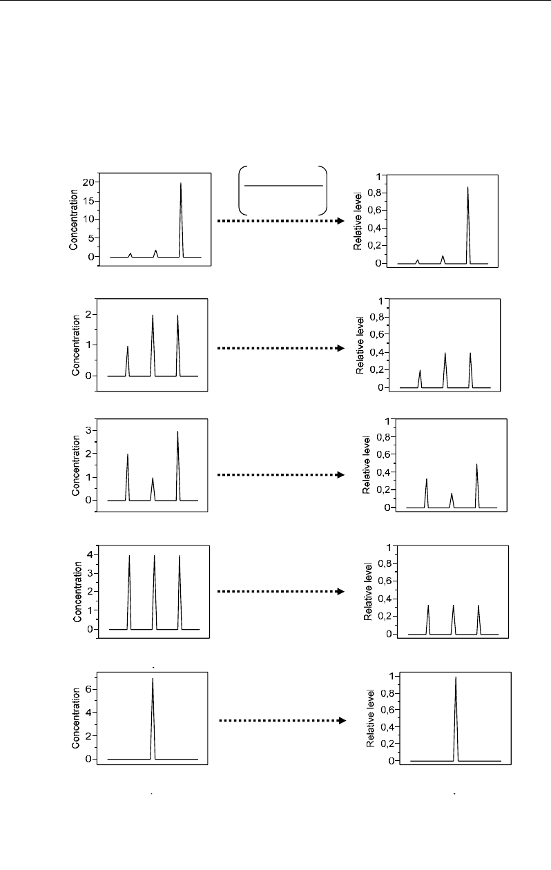
In other word, CA considers each value not by its absolute but by its relative level both

along its row and column (Figure 59): for example, in individuals X3 and X4, the absolute

values (e.g. concentration) of variable M3 (e.g. metabolite M3) are equal to 3 and 4,

respectively, leading to consider the second as more important than the first. However, in

terms of relative values, the 3 of X3 and the 4 of X4 represent 50% and 33%, respectively, of

the total in their profiles; consequently, the value 3 of profile X3 is relatively more important

than the value 4 in profile X4, leading to consider individual X3 as more associated than X4

to variable M3. However, by considering all the individuals X1 to X5, the relative level 50%

of M3=3 in its profile appears to be lower than that M3=20 in X1 (87%). Individual X1

appears finally as the most associated to variable M3 by considering all the rows (profiles)

and columns (variables) of the dataset. To conclude on the outlier or non-outlier state of X1,

all the individuals X

of the dataset must be considered according to all the variables; this

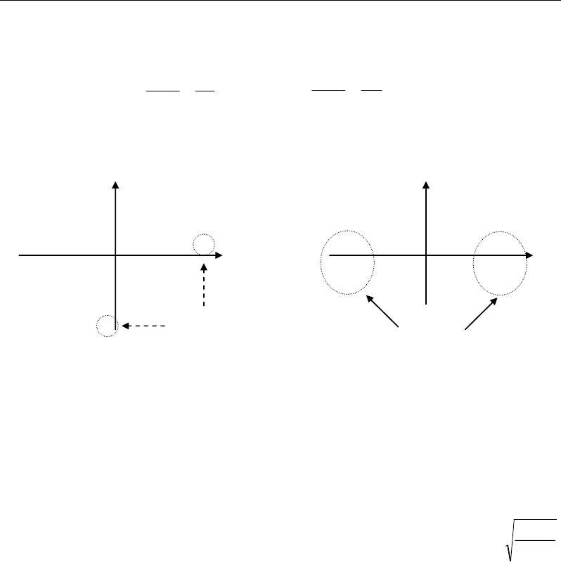
allows to check if X1 is alone to be original (a), or if the other individuals are also original

under other characteristics (b). In the first case (a), the rarity of X1 makes to consider it as

atypical; in the second case (b), one talks about different trends in the dataset rather than

atypical cases (or outliers) (Figure 60).

Nabil Semmar 72

V.6.3.2 Basic Computations in Correspondence Analysis

Correspondence analysis (CA) is an exploratory multivariate method which analyses the

relative variations within a simple two-way table X (n rows × p columns) containing

measures of correspondence between rows and columns. The matrix X consists of additive

data both along the rows and columns (e.g. contingency table, concentration dataset, or any

homogeneous unit matrix). Thus, CA analyses simultaneously row and column profiles.

M1 M2 M3

Metabolites

M1 M2 M3

Concentration

Sum of

Concentrations

M1 M2 M3

Metabolites

M1 M2 M3

Figure 59. Standardization of concentration (absolute values) profiles into relative levels leading to data

homogeneization at a scale varying between 0 and 1.

Correlations - and Distances - Based Approaches to Static Analysis… 73

Row and column profiles are obtained by dividing each value x

(e.g. concentration of

metabolite j in subject i) by its row and column sums, x

and x

respectively:

∑

(j=1 to p)

∑

(i=1 to n) (eq. 4)

Atypical

points

× ×

Two opposite

trends

(a) (b)

Figure 60. Illustration of two dataset structures corresponding to the presence of isolated atypical

individual cases (a) and to grouped individuals into well distinct trends (b).

This transformation is appropriate to highlight the strongest associations between rows

and columns: two row profiles are more similar if they show comparable relative values for

the same column-variables. Reciprocally, two variables will have similar variation trends if

their relative values vary in the same way in all the rows. Finally, a row i is strongly

associated with a column j if it has a high value x

for this column compared with all the

values both of the same row i and of the same column j. This duality along row and column

leads to standardize each value x

by the square root of the product of x

and x

(Figure 61).

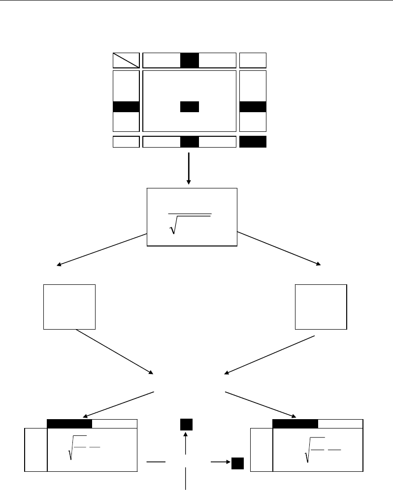
From the matrix T of such standardized values, two analyses are performed to calculate

new coordinates (called factorial coordinates) for rows (individuals) and columns (variables),

respectively (Figure 61). Row analysis is performed on the matrix T’T, whereas column

analysis is performed on the matrix TT’. One obtains two squared matrices TT’ and T’T

which have (p-1) eigenvalues λ

comprised between 0 and 1; p being the smallest dimension

of the dataset (generally, in a dataset (n × p), there are less variables than individuals, i.e.

p<n). Extreme eigenvalues equal to 0 or 1 are not considered because they correspond to

trivial values.

The (p-1) decreasing eigenvalues λ

are combined with the matrices T’T on the hand and

TT’ on the other hand, to calculate (p-1) eigenvectors V

for the rows and for the columns,

respectively. Finally, the factorial coordinates of the rows and columns are calculated from

the scalar products of eigenvectors by:

- the row profiles (x

) weighted by the root square of the ratio x

- the column profiles (x

) weighted by the the root square of the ratio x

Nabil Semmar 74

The new coordinates resulting from row and column analyses have the characteristic to

condense the variability of the initial dataset within a small dimension space (<p) consisting

of independent directions (called factors). The factors have also the property to be

successively shorter because they correspond to decreasing eigenvalues; this makes possible

to describe the variability of the initial dataset by a minimal dimension space represented by

the first factors (Escofier and Pagès, 1991): the first factor (F1) describes the maximal part of

total variability followed be the second (F2) which describes a maximal part of the remaining

variability not described by F1, etc. . This leads the variability of the dataset to be rapidly

condensed into a small dimension space. This is particularly interesting in the case of large

datasets, what is generally the case in metabolomics.

The computations of factorial coordinates are illustrated by a numerical example based

on the previous dataset (Figure 55) (Figures 62, 63). After the calculus of factorial

coordinates of the rows along each factor, their sign must correspond to those of the

coordinates of the eigenvectors for the columns: for instance, along F1, the eigenvector of

column is V1 with five coordinates (0.58, -0.12, 0.07, -0.17, -0.78) (Figure 63); the calculus

of factorial coordinates of the five rows along F1 gives (-0.59, 0.27, -0.14, 0.24, 1.44); as the

two sets have opposite signs, it is needed to multiply one of them by -1 to obtain appropriate

superimposition between rows and columns: Thus F1 becomes F1(0.59, -0.27, 0.14, -0.24,

-1.44) (Figure 62). According to the dataset, such sign correction can or can’t occur.

To measure the distance between two row-profiles or two column-profiles, CA uses the

chi-square distance. The distance between two row profiles (e.g. two patients) i and i’ is given

by (Escofier and Pagès, 1991; Greenacre, 1984; 1993):

∑

+++

⎟

⎠

⎞

⎜

⎝

⎛

−=

iid

)',(

(eq. 5),

where x

is the total sum of the whole database, x

, x

i’+

are the sums of rows i and i’,

respectively, and x

is the sum of column j.

This distance is low when the profiles show similar relative values of several variables,

independently of their absolute values (Figure 45). Similarly, the distance between two

column profiles (e.g. two metabolite variables) j and j’ is given by:

∑

+++

⎟

⎠

⎞

⎜

⎝

⎛

−=

jjd

)',(

(eq. 6)

V.6.3.3. Graphical Interpretation of CA Results and Outlier Diagnostic

Graphical visualization of the factorial coordinates of rows helps to see how much each

individual tends to be original or ordinary within the population. Moreover, the scatter plot of

the factorial coordinates of columns helps to identify how the different variables are

associated to original individuals: an individual which projects close to a variable means a

high value in such individual for such a variable compared with all the individuals and

variables of the dataset. Graphically, outliers can be highlighted by extreme points along the

Correlations - and Distances - Based Approaches to Static Analysis… 75

factors (computed axes) of CA (Greenacre, 1984, 1993). Moreover, the duality in CA allows

identification of the variables responsible of the outlying states of such individuals.

1…

…

Sum

…

… …………… …

…

… …………… …

…

Sum

…

Row analysis Column analysis

T’T TT’

p × p n × n

p eigenvalues

p eigenvectors V

F1 F2 …

…

⎥

⎦

⎤

⎢

⎣

⎡

F1 F2 …

…

⎥

⎦

⎤

⎢

⎣

⎡

V ..

Visualization

Factorial coordinates of n rows Factorial coordinates of p columns

Figure 61. Principle of computation of factorial coordinates in correspondence analysis.

From the numerical example, the individuals X1 and X5 showed opposite and extreme

projections along F1 (first factor) (Figure 62). Morever, long F1, the variables M3 and M2

projected in the same spaces than X1 and X5, respectively (Figure 63); this indicates that

individuals X1 and X5 have relatively high values of M3 and M2, respectively, by

comparison with all the values of the corresponding row and column profiles: in fact, the

values: M3=20 in X1 and M2=7 in X5 represent high maxima both along their rows and

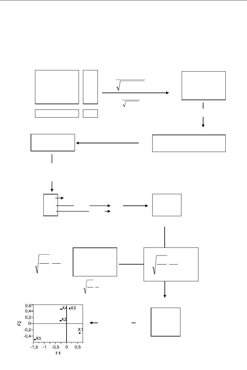
Nabil Semmar 76

columns. The opposition between X1 and X5 can be explained by an inverse variability of

M2 and M3 between X1 and X5: X1 has a high M3 and a low M2, whereas X5 shows inverse

characteristics. Moreover, the pair (X5, M2) appears more extreme along F1 than (X1, M3).

This is due to the fact that the value 7 of M2 in X5 is relatively more important than the value

20 of M3 in X1: 100% versus 87%.

M1 M2 M3

1220

122

213

444

070

81629 53

e.g.

07.0

823

Transposition

0.07 0.10 0.77

0.16 0.22 0.17

0.29 0.10 0.23

0.41 0.29 0.21

0.00 0.66 0.00

0.07 0.16 0.29 0.41 0.00

0.10 0.22 0.1 0.29 0.66

0.77 0.17 0.23 0.21 0.00

T’=

T’.T

0.07

0.10 + 0.16

0.22 +

0.29×0.10 + 0.41×0.29 +

0×0.66 = 0.19

e.g.

T’T=

Diagonalization of T’T:

determination of eigenvalues

λ then eigenvectors V

0.28 0.19 0.24

0.19 0.59 0.20

0.24 0.20 0.72

Trivial value

1.00

0.45

0.15

=0.45

=0.15

V1 V2

0.04 0.92

0.79 -0.27

-0.61 -0.29

Eigenvectors V

Eigenvalues

⎥

⎦

⎤

⎢

⎣

⎡

0.11 0.16 1.18

0.51 0.73 0.54

0.86 0.30 0.68

0.86 0.61 0.45

0.00 1.82 0.00

e.g.

73.0

⎥

⎦

⎤

⎢

⎣

⎡

Factorial

coordinates

0.11

0.92 + 0.16×(-0.27)

+ 1.18×(-0.29) = -0.28

e.g. :

Visualization

F1 F2

0.59 -0.28

-0.27 0.13

0.14 0.52

-0.24 0.50

-1.44 -0.48

Figure 62. Numerical example illustrating the computation of factorial coordinates of rows in

correspondence analysis (row analysis).