Knapp J.S., Cabrera W.L. Metabolomics: Metabolites, Metabonomics, and Analytical Technologies
Подождите немного. Документ загружается.

Correlations - and Distances - Based Approaches to Static Analysis… 37
correlation matrix) is a global property of the metabolic system, i.e. whether two metabolites are
correlated or not does not depend solely on the reactions they participate in, but on the
combined result of all the reactions and regulatory interactions present in the system. In this
sense, the pattern of correlations can be interpreted as a global fingerprint of the underlying
system integrating environmental conditions, physiological states, etc., at a given time.
Apart from the temporal, physiological and environmental factors, the correlation
between two metabolites can show a scale-dependent variation within a same metabolic
system; this provides evidence on the flexibility of metabolic processes and on the complexity
of metabolic network:
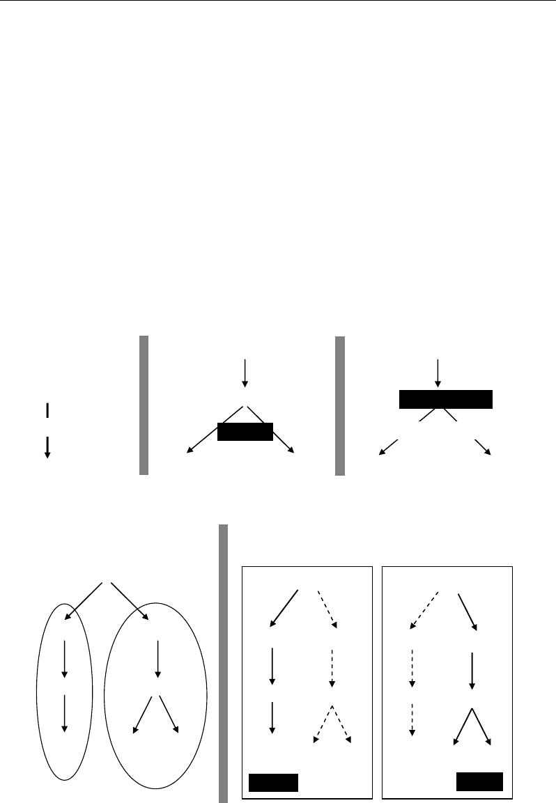
At a local scale, two metabolites are closely considered the one toward the other without
consideration of the other metabolites. For example, two metabolites can be competitive for a
same enzyme (Figure 32b) or a same precursor (Figure 32c) within a common metabolic
pathway leading to a locally negative correlation between them. However, when they are
considered together into their common pathway in presence of other competitive pathways,
these two metabolites can manifest a positive correlation at the global scale (Figure 32d:
Metabolites M7, M8).
M1 (precursor)
M2 (product)
M1 (precursor)
M2
(product)
M1 (precursor)
M2
(product)
M3
(product)
Enzyme
Enzyme B Enzyme A
Enzyme
(a)
(b)
(c)
M1
M2
M5
M3
M4
M7
M8
M6
Pathway A Pathway B
M1
M2 M5
M3
M4
M7 M8
M6
Path. A
M1
M2 M5
M3
M4
M7 M8
M6
Path. B
Path. A
Path. B
(d) (e)
M3
(product)
Figure 32. Different scales at which correlation between metabolites can be interpreted: metabolite
scale (a-c); metabolic pathway scale (d); Network (physiological) scale (e).
Nabil Semmar 38
Two
dominant
p
ara
m
eters
One
dominant
p
arameter
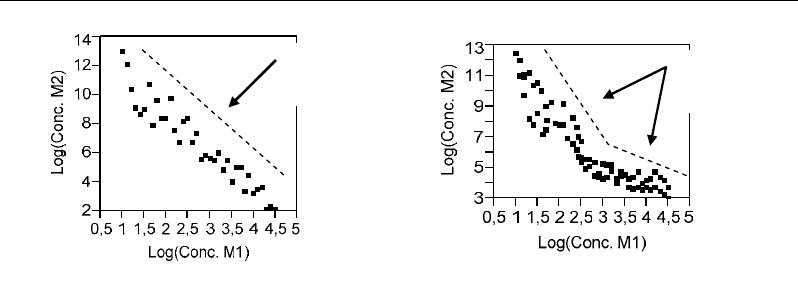
Figure 33. Some examples of Log-Log scatter plots used to detect co-response of two metabolites under
the effect of some dominant parameter(s).
At a global scale, several metabolites can be biosynthesized within a same metabolic
pathway in which they share a serial of regulation enzymes, by competting other metabolites
belonging to other metabolic pathways (Figure 32d).
At a higher scale, diminutive fluctuations within the metabolic system or in the
environment conditions induce correlations which will propagate through the system to give
rise to a specific pattern of correlations depending on the physiological state of the system
(Camacho et al., 2005; Steuer et al., 2003a, b; Morgenthal et al., 2006) (Figure 32e).
A transition from a physiological state to another may not only involve changes in the
average levels of the measured metabolites but additionally may also involve changes in their
correlations.
There are many pairs of metabolites that are neighbours in the metabolic map but which
have low correlations, and others that are not neighbours but have high correlations. This is
due to the fact that the correlations are shaped by both stoichiometric and kinetic effects
(Steuer et al., 2003a, b).
IV.1.6. Multidimensional Correlation Screening by Means of Principle Component
Analysis
IV.1.6.1. Aim
Principle component analysis (PCA) is a multivariate analysis which uses the linear
algebra rules to provide graphical representations where the n rows and p columns of a
dataset will be restricted to n and p points, respectively, on a single axis or in a plan (Waite,
2000). PCA aims to represent the complexity of relationships between variables in the
minimum number of dimensions. The relative positions of row- and column-points given by
PCA are interpretable in terms of affinities, oppositions or independences between them; this
helps to understand:
- specific characteristics of individuals (e.g. metabolic profiles),
- relative behaviours of variables (e.g. metabolites),
- associations between individuals and variables.

Correlations - and Distances - Based Approaches to Static Analysis… 39
M3
M1
M2
M4
×
M4
M3
×
×
M1
M2
×
×
M1
M3
M2
×
M4
F2
F1
Orthogonal decomposition
Successive perpendicular axes
Total variability space
Figure 34. Simplistic illustration of decomposition of the total variability into additive (complementary)
parts along perpendicular axes.
F1
F2
F3
Figure 35. Intuitive illustration of the usefulness of orthogonal decomposition to describe a complex
variability according to decreasing complementary parts (Fj).
Nabil Semmar 40
In the plan, row-points can show grouping into different “constellations” indicating the
presence of different trends or sub-populations in the dataset.
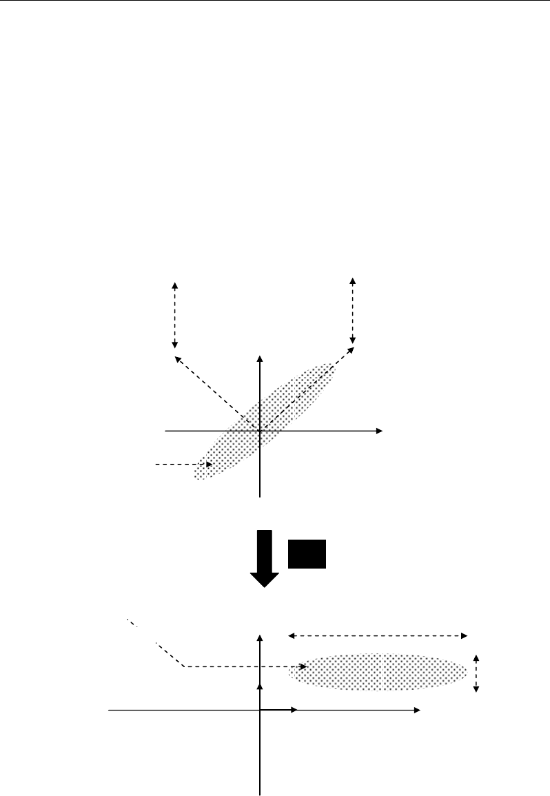
For that, PCA decomposes the variability space of a dataset into a succession of
orthogonal axes representing decreasing and complementary parts of the total variability
(Figure 34). From the simplistic illustration, decomposition of the total variability into two
orthogonal directions F1 and F2 highlights clearly some similar and opposite behaviours of
the different variables M
j
: along F1, the variables M1 and M2 show a certain affinity and
seem to be opposite to the variables M3 and M4 (projected on the other extremity of F1).
Such information is completed by that along F2 where M1 and M3 share a similar behaviour
opposite to that of the variables M2 and M4.
This illustrates the aim of PCA consisting in handling the complex variability under
successive complementary view angles.
F1
F2
λ
1
λ
2
U
1
U
2
eigenvalue
eigenvector
Principle
component
Data variability
under two
orthogonal angles
Initial
Variable M
j
Initial
Variable M
j’
Better directions for variability analysis
PCA
Data variability in
the initial
multivariate space
F1
F2
Figure 36. Graphical illustration of principle of PCA based on calculation of eigenvalues
λ
k
,
eigenvectors U
k
and principle components F
k

Correlations - and Distances - Based Approaches to Static Analysis… 41
IV.1.6.2. General Principle of PCA
PCA is a decomposition approach based on the extraction of the eigenvalues and
eigenvectors of a dataset. The eigenvectors give orthogonal directions called the principle
components (F
j
) which describe complementary and decreasing parts of the total variability
(Figure 35).
The decrease in explained variability is closely linked to the eigenvalues sorted by
decreasing order. To each eigenvalue λ
j
of the dataset corresponds an eigenvector U
j
which
gives the direction of principle component F
j
; the variability explained along F
j
is equal to λ
j
and it can be expressed in terms of relative part by λ
j
/∑(λ
j
) (Figure 36) (Waite, 2000).
IV.1.6.3. Computation of Eigenvalues, Eigenvectors and Principle Components
Eigenvalues and eigenvectors are calculated for a square (p × p) and invertible (i.e. not
null determinant) matrix A. Therefore, any square matrix A (p × p) can be decomposed into p
directions F
k
defined by p eigenvectors U
k
and weighted by p eigenvalues
λ
k
. From an
experimental dataset X, a square matrix A can be directly obtained by the product A= X’X;
therefore, the eigenvalues and eigenvectors are calculated from A.
The eigenvalues
λ
k
and their corresponding eigenvectors U
k
are calculated for a square
matrix A (p × p) by solving the following matricial equation:
A.U = λ.U ⇔ A.U - λ.U = 0 ⇔ (A - λ.I). U = 0 ⇔ (A - λ.I) = 0
where I is a (p × p) identity matrix: I =
1
0…00
0
1
…0 0
00
1
00
00…
1
0
00…0
1
1 … … … p
1
.
.
.
p
This matricial equation is solved by setting its determinant to zero: det(A - λ.I) = 0, leading to
solve a p equation system with p unknown λ
k
. After computation of the eigenvalues
λ
k
, the
corresponding eigenvectors U
k
are calculated from the initial equation A.U = λ.U.
Finally, from the eigenvectors U
k
, the initial variables M
j
of the dataset X are replaced by
“synthetic” variables F
k
(called principle components) obtained by linear combinations of the
p initial variables M
j
affected by the coordinates of the corresponding eigenvectors U
k
:
pkipjkijkikiki
p
j
jkijik
uxuxuxuxuxUXF ...........
332211
1
++++++==
∑
=
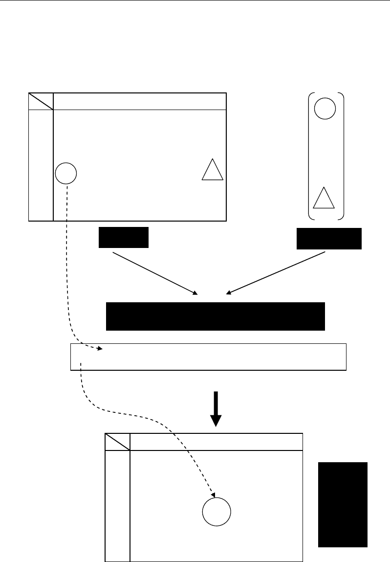
In other words, from the p coordinates x
ij
of a row i corresponding to the p columns j, one
new coordinate F
ik
is calculated to represent the new position of row i along the principle
component F
k
(Figure 37). The new coordinates, called factorial coordinates, are more
Nabil Semmar 42
appropriate to associate behaviours of different individuals i to some levels of variables M
j
,
leading to understand the variability structure of the initial dataset X.
To understand more the calculation and the interpretation of eigenvalues, eigenvectors
and factorial coordinates in PCA, let’s give a simplistic numerical example based on a square
matrix A (2 × 2).
i
j
M
1
M
2
M
3
…
M
j
…
M
p
id 1
id 2
:
:
:
id i
x
i1
x
i2
x
i3
…
x
ij
…
x
ip
:
:
:
id n
F
ki
= x
i1
×u
1k
+ x
i2
×u
2k
+ x
i3
×u
3k
+ … + x
ij
×u
jk
+ … + x
ip
×u
pk
u
k1
u
k2
u
k3
:
:
u
kj
:
u
kp
Dataset X
Eigenvector U
k
New coordinate of the row i along the principle
component F
k
defined by the eigenvector U
k
×
i
k
F
1
……
F
k
……
F
p
id 1
id 2
:
:
:
id i
F
i1
……
F
ik
……
F
ip
:
:
:
id n
New
coordinates
of rows i
along
principle
components
F
k
Figure 37. Computation of new coordinates (factorial coordinates) of an individuals i along a principle
component F
k
by a linear combination of its initial coordinates x
ij
affected by the coordinates of the
eigenvector U
k.
Correlations - and Distances - Based Approaches to Static Analysis… 43
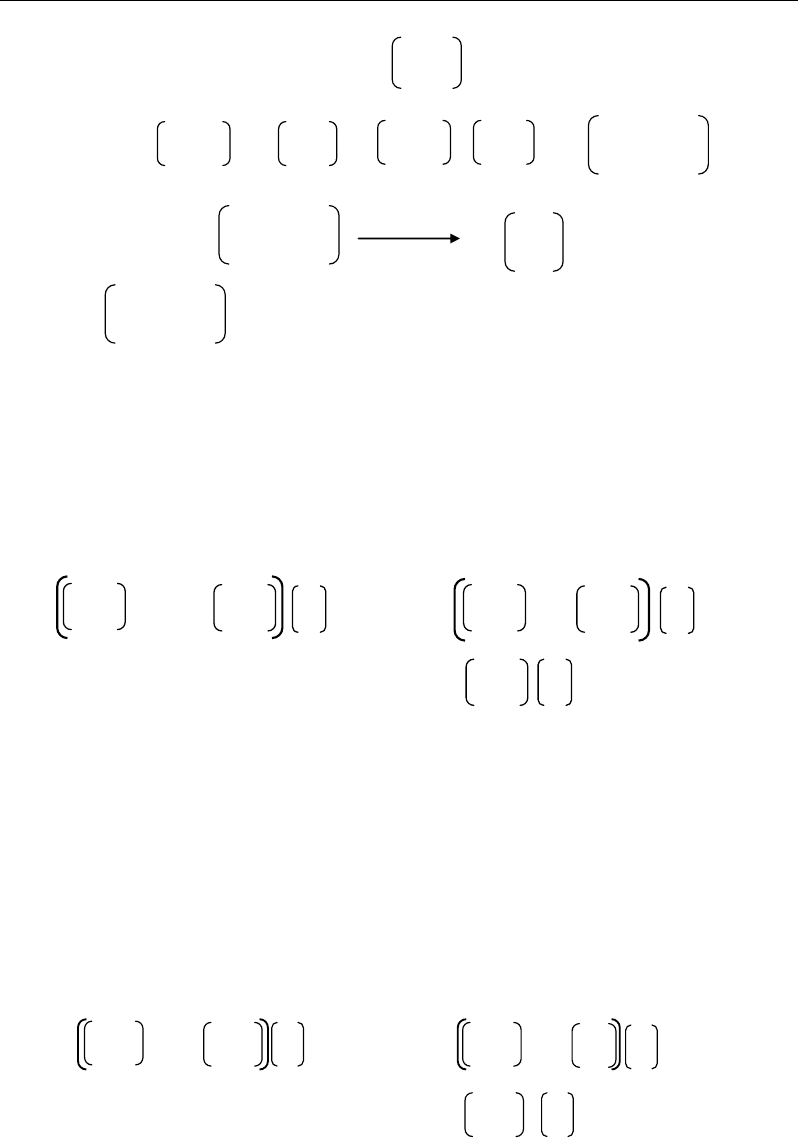
A - λ.I = - λ = - =
det (A - λ.I) = det det = ad – bc
det = [(2 - λ)(-6 - λ) – 9] = λ² + 4λ -21
A =
23
3-6
23
3-6
10
01
23
3-6
λ
0
0
λ
2 -
λ
3
3
-6 -
λ
2 -
λ
3
3
-6 -
λ
ac
bd
2 -
λ
3
3
-6 -
λ
Setting λ² + 4λ -21 to 0 leads to the equivalent form: (λ - 3)(λ + 7) = 0, so the
eigenvalues λ
k
of A are 3 and -7. After sorting these two λ
k
by decreasing absolute value, we
have λ
1
= -7 and λ
2
= 3.
For each eigenvalue λ
k
, the corresponding eigenvector U
k
is calculated by solving the
matricial equation (A - λ.I).U = 0:
For λ
1
= -7, the matricial equation will be:
= 0 ⇔ = 0
⇔ = 0
23 10u
11
3-6-(-7)01 u
21
23
70
u
11
3-6
+0
7u
21
93
u
11
31
u
21
This leads to the following equation system:
9u
11
+ 3u
21
= 0 ⇔ 9u
11
= -3u
21
3u
11
+ u
21
= 0 ⇔ 3u
11
= -u
21
For u
11
= 1, we have u
21
= -3. Therefore, U
1
= (1, -3) is the first eigenvector of A.
Note that due to the fact that the equation system is reduced to one equation with two
unknown, results in the existence of infinity of eigenvectors proportional to U
1
.
For λ
2
= 3, the matricial equation will be:
= 0 ⇔ = 0
⇔ = 0
23 10u
12
3-6
-
(-3) 0 1 u
22
23
30
u
12
3-6
+
0
3u
22
-1 3
u
12
3-9
u
22
(3) -
This leads to the following equation system:
-u
12
+ 3u
22
= 0 ⇔ u
12
= 3u
22

Nabil Semmar 44
3u
12
- 9u
22
= 0 ⇔ 3u
12
= 9u
22
For u
22
= 1, we have u
12
=3. Therefore, U
2
= (3, 1) is the second eigenvector of A.
Also, the fact that the equation system is reduced to one equation with two unknown
results in the existence of infinity of eigenvectors proportional to U
2
.
The two calculated eigenvectors U1 and U2 define a new basis of orthogonal directions
along which the row and column variability of the dataset A can be topologically analysed
(Figure 38).
3
1
-3
1
Initial variability
axis j
Initial variability
axis j’
U
2
U
1
Figure 38. Illustration of the orthogonality between the eigenvectors of a matrix.
After calculation of the eigenvectors U
1
and U
2
, the new coordinates F
ik
of the rows i
along the principal components k (k=1 to 2) can be calculated by the scalar product A.U
k
.
Thus, along the principle component F1 defined by the direction of U1, the two rows of the
matrix A will be represented by two coordinates given by:
A.U
1
=
23 1
3-6 -3
-7
21
; this result is also obtained by the product λ
1
.U
1
.
Along the second principle component F2, each row of the matrix A will have a new
coordinate given by:
A.U
2
=
23 3
3-6 1
=
9
3
; this result is also obtained by the product λ
2
.U
2
.
Finally, the dataset A can be replaced by the new matrix F giving the factorial
coordinates of the rows (individuals) i along each principle component F
k
(k=1-2):
F =
-7 9
21 3
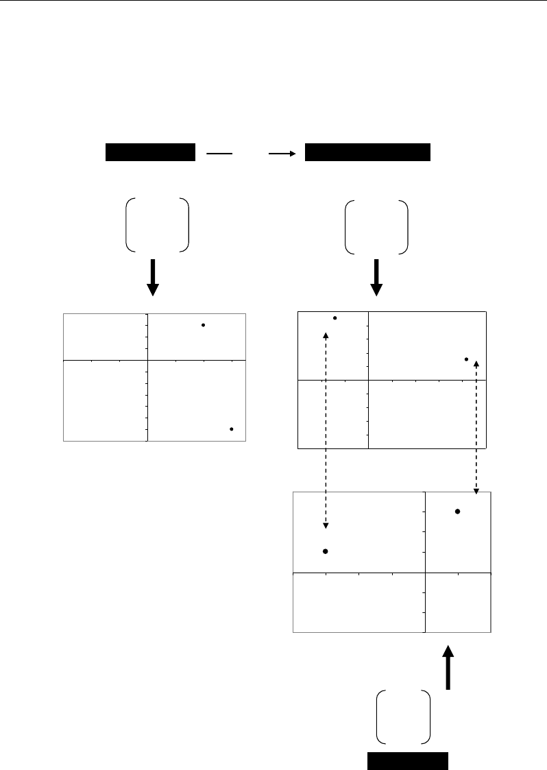
; from F, the individuals (the rows) of the dataset A can be projected on the
plane F1F2 for a topological analysis of their variability (Figure 39). To link the variability of
individuals to that of variables, a variable plot can be obtained from the coordinates of the
eigenvectors by which the initial variables were weighted (Figure 39). According to their
absolute values, such coordinates attribute more or less importance to the initial variables Mj
in the new (factorial) coordinates of individuals i. For example, the individual id1 has a
factorial coordinate equal to -7 on F1; this value was calculated by the following linear
combination:
-7 = (id1).U1 = (2 3) = (2 × 1) + (3 × -3 )
1
-3
=
Correlations - and Distances - Based Approaches to Static Analysis… 45
In this linear combination, the second variable M2 is affected by an eigenvector score
equal to -3 the absolute value of which (Abs(-3)=3) is higher than the coordinate=1 by which
is affected the first variable M1. This remark concerning the role of M2 on F1 can be
generalised for all the factorial coordinates along F1. This helps to conclude that the
variability of all the individuals on F1 is mainly due to the variable M2. Graphically, this can
be showed by a projection of M2 both at extremity and close to the axis F1 (Figure 39).
M1 M2
id 1
23
id 2
3-6
Initial variables
Individuals
Initial dataset A Factorial coordinates
F1 F2
id 1
-7 9
id 2
21 3
Principle components
Individuals
-7
-6
-5
-4
-3
-2
-1
0
1
2
3
4
-3 -2 -1 0 1 2 3
Variable M1
Variable M2
id 1
id 2
-10
-8
-6
-4
-2
0
2
4
6
8
10
-15 -10 -5 0 5 10 15 20 25
Principle component F1
Principle component F2
id 1
id 2
Individuals’ plot
PCA
Eigenvectors
Variables
-3
-2
-1
0
1
2
3
4
-4 -3 -2 -1 0 1 2
Eigenvector U1
Eigenvector U2
Variables’ plot
M1
M2
U1 U2
M1
13
M2
-3 1
Figure 39. Graphical analysis of links between the variability of individuals and that of variables by
means of PCA.

Nabil Semmar 46
IV.1.6.4. Graphical Interpretation of Factorial Plans
According to the factorial plan F1F2 of individuals (Figure 39), id1 and id2 show
opposition along F1. According to the variable plot, the variables M1 and M2 seem to be
opposite, and projected on the same sides than id2 and id1, respectively. Taking into account
the importance of variable M2 on F1, and the graphical proximity between M2 and id1, the
opposition of id1 to id2 can be explained by a high value of M2 in id1 and a low one in id2.
In fact, the initial dataset A shows values of 3 and -6 for M2 in id1 and id2, respectively.
Thus, the PCA helped to identify that the highest variability source in the dataset A consisted
of an important opposition between id1 and id2 for variable M2. In metabolomic terms, this
can correspond to a situation where some individuals are productive of a metabolite M2
whereas others are relatively deficient in M2.
For F2, the highest coordinate of corresponding eigenvector U2 concerns variable M1,
leading to deduce that the role of M1 on F2 is relatively more important than that of M2.
Graphically, the individual id2 projects closer to M1 than it is id1. This translates a higher
value of M1 in id2 than in id ; this can be checked in the initial dataset A. From this simplistic
example, variable M2 appears to play a separation role between individuals (profiles),
whereas the variable M1 seems to group the individuals according to a more or less affinity.
The fact that id1 and id2 are bot opposite alonf F2 can be attributed to their relatively close
positive values (2 and 3, respectively).
Apart from the dual analysis between rows (individuals) and columns (variables), the
interpretations in PCA can be focused on the variability of variables and individuals,
separately: on the plan F1F2 (Figure 39), the variables M1 and M2 seem to have mainly
opposite behaviours from their projections in two different parts of the plan. This opposition
is observed for individuals, and seems to indicate the presence of two trends in the initial
dataset A.
IV.1.6.5. Different Types of PCA
The variability of a dataset X (n×p) can be analysed by PCA on the basis of different
criteria by considering (Figure 40):
- The crude effects of variables leading to give more importance to the most dispersed
variables from the axes’ origin.
- The variations of data around their mean vector (centered PCA) leading to analyse
the variability of the dataset around its gravity centre GC.
- Standardized data obtained by homogenizing the variation scales of all the variables
through their weighting by their variances. This leads to analyse the variability of the
dataset around the gravity centre and within a unity scale space.
- Ranked data consisting in using the ranks of data rather than their values.
- These different PCA are performed from different square matrices (p × p):
- PCA on crude data is performed on the square matrix X’X.
- Centred PCA is performed on the square matrix C’C, with
XXC −=
, and where
X
is the mean vector of the different variables.
