Knapp J.S., Cabrera W.L. Metabolomics: Metabolites, Metabonomics, and Analytical Technologies
Подождите немного. Документ загружается.

Correlations - and Distances - Based Approaches to Static Analysis… 7
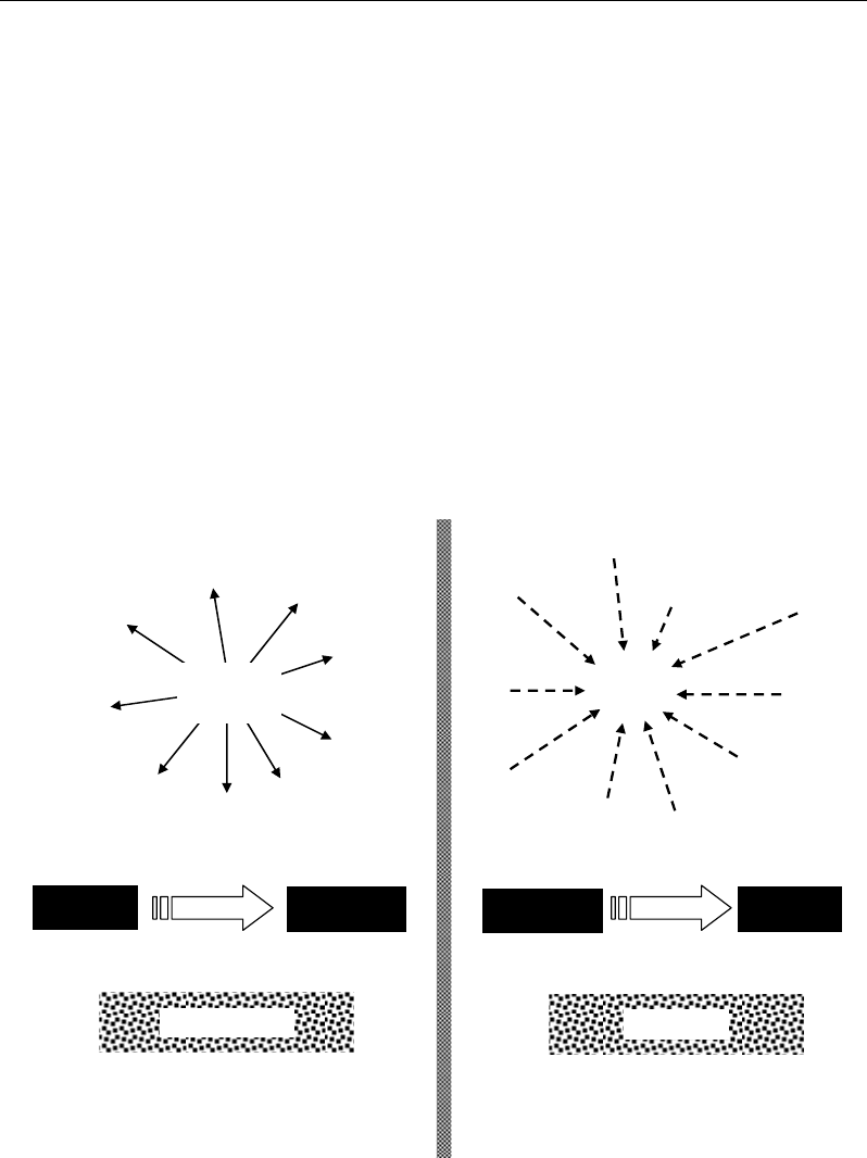
words, the descriptive approaches aim identification of different variability trends/states of
metabolic systems; for that, metabolomic datasets are analyzed in order to highlight how units
or individuals separate the ones from the others leading to multidirectional behaviours within
the system. This helps to identify substructures or system components from which the
biological (metabolic) complexity can be described. However in predictive approaches, the
steps and the aim are inverted: different variability factors are combined in order to estimate
precisely what internal state could be acquired by the system. This helps to identify the most
significant factors which control the system.
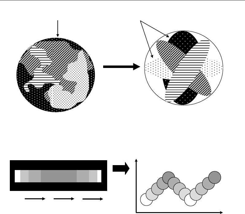
Metabolomic approaches can be also classified according to the type of datasets. Several
classifications are considered, one of the most classical consists in separating static from
kinetic datasets. These two kinds of datasets differ by the fact that the variable time is not
considered or considered, respectively. In the first case (static), a dataset is treated as a whole
block to obtain a global picture on the components or states of the system. In the second case
(kinetic), a dataset is undertaken as succession of different subsets varying in time leading to
analyze a serial of small and successive pictures representing a sequence of the system
behaviour (Figure 6).
Variability
trends
Variability
trends
Variability
trends
Variability
trends
Controllability
factors
Controllability
factors
Controllability
factors
Controllability
factors
Backbone
Background
Background
Backbone
Descriptive approaches
System
structure
System
state
Predictive approaches
Decomposition
Fusion
Figure 5. Schematic representation of the general goals of descriptive and predictive approaches.
Nabil Semmar 8
Decomposition
Filtration
Separated system
Components
Initial Static dataset Final structured dataset
(a)
(b)
Time
Kinetic/
temporal
anal
y
sis
Crude system state
Initial kinetic dataset based on
time-dependent observations
Observed serials
Highlighted/formulated time-
dependent process
Level
Figure 6. Schematic representation of static (a) and kinetic/temporal (b) analyses.
Metabolic systems are known to be complex networks in which many
components/processes are interconnected. Representations of such inter-connections require
matrix formulations which provide flexible tools to store multi-path information. On this
basis, different metabolomic approaches can be considered by reference to the matrix tool
used for metabolic system analysis. Matrix tools can be used to describe/treat distances,
correlations, connectivity, transition, reactions, equilibrium, mixtures between different
components of biological (metabolic) system (Figures 7-10, 13) (Crampin et al., 2004;
Semmar et al., 2001, 2005b, 2008 ; Sumner et al., 2003; Gonzalez-Diaz et al., 2008;
Gonzalez-Diaz, 2008; Kose et al., 2001; Llaneras and Picó, 2008; Steuer, 2007; Stelling,
2004).
This chapter will focus particularly on distance and correlation computation approaches
used for static analysis of metabolic systems. Before the detailed sections on distance- and
correlation-based approaches, a brief description of other matrix-based approaches will be
presented in the following sections, particularly on the constraint and neighbouring notions.
Correlations - and Distances - Based Approaches to Static Analysis… 9
III.2. Boolean Matrix Based Approaches
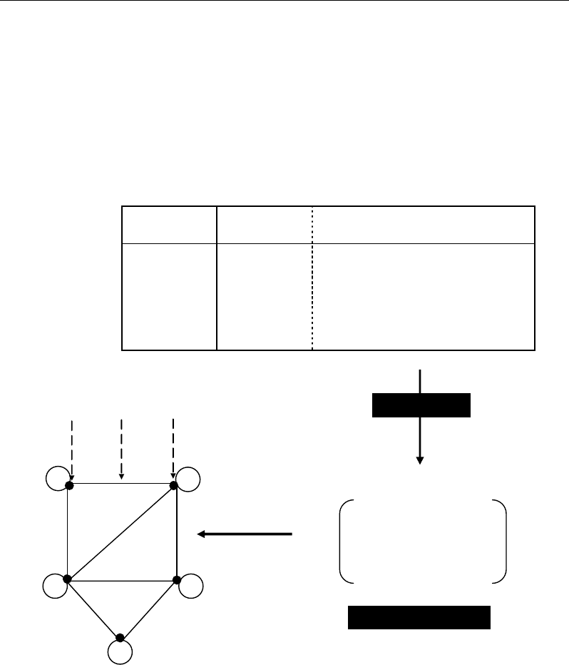
Connectivity between different (p) components of system can be codified by using a
binary formalism (Boolean code) consisting of 1 if two components are connected and 0 if
not (Estrada and Bodin, 2008; Estrada, 2006, 2007; Vilar et al., 2005; Kose et al., 2001; Janga
and Babu, 2008) (Figure 7). For instance, the value 1 can be attributed for two neighbour or
two linked metabolites (e.g. precursor-product) in the metabolic system. The resulting
adjacency matrix can be graphically represented by a multigraph containing p nodes or
vertices (corresponding to the p system components) which are connected by edges.
M1 M2 M3 M4 M5
M1
11010
M2
11110
M3 01111
M4
11111
M5 00111
Connectivities
Adjacency matrix
M1
M2
M4 M3
M5
Node
Edge
Node
Metabolites
Unchanged
states
Transformation reactions
M1 M1 → M1 M1 → M2 M1 → M4
M2
M2 → M2 M2 → M3 M2 → M4
M3
M3 → M3 M3 → M4 M3 → M5
M4
M4 → M4 M4 → M5
M5
M5 → M5
Figure 7. Boolean formalism of connectivities between metabolites in a metabolic system and
corresponding graphical representation.
III.3. Transition Matrix Based Approaches
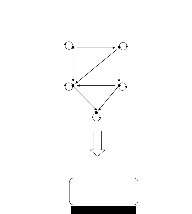
The variation of a biological (metabolic) system in time can be described by a finite
number of successive states (Guttorp, 1995; Tamir, 1998). For example, at a given time, a
metabolic system can be described by the set of the metabolites present in the network.
Between two successive times t and t+1, each molecule of metabolite j can be subjected to
different exclusive processes: it can remain unchanged, or be transformed to another
metabolite among different possible ones. The exclusivity between the different metabolic
Nabil Semmar 10
processes makes possible to analyse the evolution of the metabolic system on the basis of
probabilities of metabolites to transit between different successive states. These probabilities
(0 ≤ ≤ 1) are stored into a transition matrix the rows and columns of which represent the
initial (e.g. precursor) and final (e.g. product) elements (Figure 8).
M3
M4
M5
M1
M2
0.2
0.25
0.1
0.7
0.2
0.5
0.5
0.6
1
0.45
0.2
0.3
Final metabolite
M1 M2 M3 M4 M5
M1
0.2 0.2 0 0.6 0
Initial M2
0 0.45 0.25 0.3 0
metabolite M3
0 0 0.1 0.7 0.2
M4
0000.50.5
M5
00001
Tansition probability matrix
(Probability
that M2 gives
M
3)
=
0.
2
5
(a)
(b)
Figure 8. Basic example representing a transition probability matrix (b) and its graphical representation
(a).
III.4. Stoichiometric Matrix Based Approaches
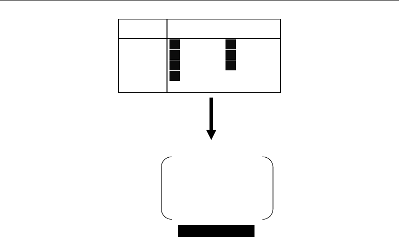
When all the metabolic reactions of a metabolic network are known, it is possible to
translate the transformation processes between precursors and products in terms of
stoichiometric coefficients. Such algebraic coefficients take positive or negative values for
appearing and disappearing metabolites, respectively. The absolute value of a stoichiometric
coefficient indicates the number of molecules implied in an elementary reaction. The set of
coefficient is stored into a stoichiometric matrix the rows and columns of which represent the
metabolites and the reactions, respectively (Figure 9).
Correlations - and Distances - Based Approaches to Static Analysis… 11
Metabolites
Transformation reactions
R
k
M1 R
1
: M1 → M2 R
2
: M1 → M4
M2
R
3
: M2 → M3 R
4
: M2 → M4
M3
R
5
: M3 → M4 R
6
: M3 → M5
M4
R
7
: M4 → M5
M5 - -
Stoichiometric matrix
R1 R2 R3 R4 R5 R6 R7
M1
-1-100000
M2
+10-1-1000
M3
00+10-1-10
M4
0+10+1+10-1
M5
00000+1+1
Metabolites
Reactions
Figure. 9. Translation of a metabolic process network into a stoichiometric matrix based on the
stoichiometric coefficients of the different metabolites for the different chemical reactions.
Stoichiometric approaches represent powerful tools for metabolic modelling when time
measurements are not available. They make possible to exploit the knowledge about the cell
metabolism structure, without considering the intracellular kinetic processes (complex and
still not well understood). Stoichiometric models have been used to (Llaneras and Picó, 2008;
Morgan and Rhodes 2002; Stelling, 2004):
- estimate the metabolic flux distribution under given circumstances in the cell at some
given moment (metabolic flux analysis) (Williams et al., 2008; Ettenhuber et al.,
2005; Kruger et al. 2003),
- predict the metabolic flux distribution on the basis of some optimality hypotheses
(flux balance analysis) (Schilling et al., 2001),
- analyse the structure of metabolism by providing information about systemic
characteristics of the cell under investigation (pathway analysis) (Schilling et al.,
2001).
Using stoichiometric matrix, the mass balance for each intracellular behavior is
disregarded with the assumption of pseudosteady state for internal metabolites. Thereby, the
mass balances can be described by a homogeneous system of linear equations. This system
constraints the flux distribution that can be achieved by the metabolic network, but it does not
predict the actual distribution. To this end, additional constraints, such as irreversibility or
capacity constraints, can be incorporated in order to determine what functional states, i.e. flux
distributions, can and cannot be achieved by a cell under certain conditions.
Nabil Semmar 12
III.5. Jacobian Matrix Based Approach
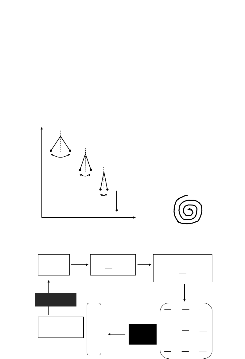
Biological (metabolic) systems can be analysed on the basis of their ability to opposite or
to be subjected to perturbations. This approach is known under the term of stability analysis
(Steuer, 2007; Fall et al., 2005):
Stability analysis aims to examine the behaviour of a system around its equilibrium state.
Equilibrium state of continue dynamical system can be represented by a stationary regimen.
The question of stability can be asked in different manners:
- If the system is deviated from the equilibrium, does it return to this state?
- Does small perturbation, moving away the system from its stationary regimen, result
in amplifications in time?
Time t
System
function
Oscillatory
stability
System with
p parameters
x
j
Variation in time
j
j
f
d
t
dx
=
Variation of the system
according to x
j
j
j
dx
df
Jacobian
matrix
(p × p)
1
1
dx
df
j
dx
df
1
p
dx
df
1
p
j
dx
df
1
dx
df
j
j
j
dx
df
1
dx
df
p
j
p
dx
df
. . . . . . . . .
. . . . . . . . .
p
p
dx
df
λ
1
λ
j
λ
p
.
.
.
.
.
.
p eigenvalues :
- real or complex
- positive or negative
Interpretation of
system stability
1
2
3
4
5
(a)
(b)
Figure 10. Basic concepts of stability analysis of dynamical systems; (a) basic example of a dynamic
stability; (b) origin, form and usefulness of Jacobian matrix in stability analysis of dynamical system.
Correlations - and Distances - Based Approaches to Static Analysis… 13
Such questions imply the analysis of all the possible perturbations of the system in
relation to small variations of its variables in time (Figure 10a). In other words, we have to
analyse the stability of a system in relation to its parameters x
j
(e.g. metabolites’
concentrations) varying in time (Figure 10b):
At equilibrium point, the derivatives of all the parameters x
j
with respect to time are null:
0==
d
t
dx
f
j
j
.
From the analytical form of f
j
, the equilibrium point x
j
* for each parameter j will be
calculated. With p parameters x
j
(j=1 to p), one expects p values x
j
* to calculate from p
derivative equations f
j
=0. Moreover, the p functions f
j
will be derived with respect to each x
j
(one at once), resulting in (p × p) partial derivatives. The set of all the partial derivatives
j
j
dx
df
is called Jacobian matrix (p × p) (Figure 10b3).
From the Jacobian matrix J, the stability of the system around the equilibrium point is
analysed. For that, all its partial derivatives are calculated at the equilibrium values x
j
* to
obtain the Jacobian matrix J*. Therefore, stability analysis of the system consists in:
- Calculating the eigenvalues λ
j
of J* (there are as much eigenvalues as parameters)
(Figure 10b4), and
- Interpreting their natures and their signs in terms of stability or non-stability of the
system (Figure 10b5).
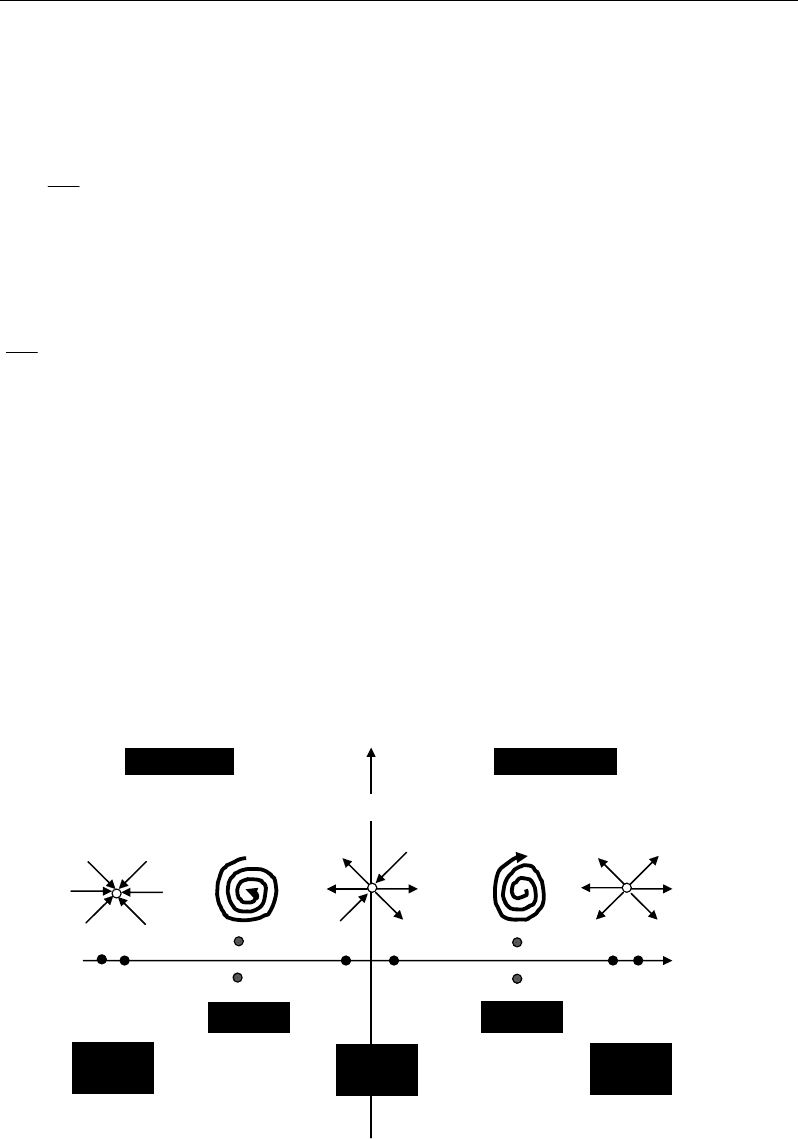
Eigenvalues of a biological (metabolic) system can be real or complex on the hand, and
positive or negative on the other hand (Figure 11):
Real
eigenvalue
Complex
eigenvalue
Oscillatory
Non
Oscillatory
Stable s
y
stems Unstable s
y
stems
(a) (b) (c) (d)
(e)
Non
Oscillatory
Non
Oscillatory
Oscillatory
Figure 11. different equilibrium states of a dynamical system interpreted according to nature and sign of
the eigenvalues of Jacobian matrix.

Nabil Semmar 14
Complex eigenvalues indicate an oscillatory system (Figure 11b, d). Inversely, a system
with only real eigenvalues is non-oscillatory (Figure 11a, c, e). Therefore, the sign of
eigenvalue provides information on the convergence or divergence of the system, i.e. on its
stability or non-stability, respectively: a negative real eigenvalue (or real part) indicates a
stable system, i.e. a system which converges (returns) to steady state (equilibrium) (after
disruption) (Figure 11a, b). A positive real eigenvalue (or real part) indicates an unstable
solution which means that the system never converge to steady state (Figure 11d, e). When
some eigenvalues are positive and others are negative, the system has a sell point, which
represents a fragile equilibrium state leading the system to be unstable (Figure 11c).
III.6. Scheffe Matrix Based Approach
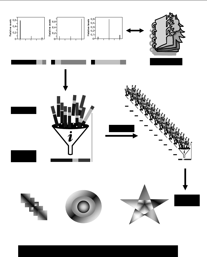
Metabolic system can be undertaken under a background consisting of different observed
regulation patterns issued from a common metabolic backbone considered as a central black
box. Such patterns represent extreme metabolic trends which are characterized by more or
less high regulation ratios of some metabolites due to more or less high expressions of some
metabolic pathways (Figure 12a). Therefore, any observed metabolic profile can be
considered as more or less closer to one of these metabolic patterns. Statistically, any
observed profile can be expressed by a particular combination of the extreme patterns
affected by appropriate weights: the variation of the combined pattern weights leads to a set
of combinations corresponding to different average patterns (Figure 12b); such mixture-
resulting average patterns will be more or less close to the different observed profiles. Under
a chemical aspect, the combination of different patterns can be assimilated to a
concentration/dilution process where the more weighted patterns will be concentrated and the
less ones will be diluted in the mixture.
After iterations of the complete set of combinations (Figure 12c), a response matrix of
smoothed profiles is obtained by averaging the repeated average profiles’ matrices (Figure
12d). Such a final smoothed data matrix is then used to analyze graphically the metabolic
processes which would be responsible for the observed polymorphism (Figure 12e). More
details are given in Figures 13 and 14.
The complete set of linear combinations of extreme states (or basic components) can be
formalised by a mixture design represented by Scheffe matrix (Figure 13) (Sado and Sado,
1991; Scheffe, 1958, 1963; Duineveld et al., 1993). The total number N of combinations to
carry out depends on two parameters: (i) the number of components (patterns) to combine and
(ii) the number n (constant) of elements (e.g. metabolic profiles) to mix in each combination.
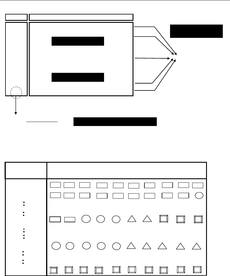
An illustration of the Scheffe matrix is given for q=4 components and n=10 elements
representing the q components in each mixture (Figure 13b). Each combination can be
summarized by an average profile (Figure 14a). The mixture design is iterated several times
to take into account the variability of the observed metabolic profiles (Figure 14b). From k
iterations, a final response matrix containing a complete set of smoothed metabolic profiles is
calculated by averaging all the k response matrices (Figure 14c). This smoothed final
response matrix can be used to graphically analyse the variability between regulation ratios of
different metabolites in order to understand metabolic processes responsible for the observed
polymorphism (Figure 14d):
Correlations - and Distances - Based Approaches to Static Analysis… 15
Metabolites Metabolites Metabolites
Classification
Mixtures
Single
Average
Iteration
Smoothed
average
Graphical analysis of smoothed metabolic profiles to identify regulation
processes responsible of observed polymorphism
Monotonous processes Cyclic processes Scale dependent processes
(c)
(b)
(a)
1 … j … p 1 … j … p
1 … j … p
(d)
(e)
Figure 12. Schematic representation of the steps of metabolomic approach consisting in iteratively
combining observed metabolic profiles representing different patterns to obtain a dataset of smoothed
profiles helping to analyse graphically the regulation processes responsible of the observed chemical
polymorphism (Semmar et al., 2007; Semmar, 2010).
As the observed patterns represent a background of the metabolic system, their iterative
combinations can provide a way to access to a backbone of such common system. On the
basis of this concept, a new metabolomic approach was developed from which the flexibility
of metabolic regulations was graphically highlighted (Semmar et al., 2007; Semmar, 2010).
Nabil Semmar 16
Mixtures Pattern 1 …
Pattern
j
…
Pattern
q
1
n
11
…
n
1j
…
n
1q
:
:::::
:
:::::
i
n
i1
…
n
ij
…
n
iq
:
:::::
:
:::::
N
n
N1
…
n
Nj
…
n
Nq
cst=
∑
=
=
q
j
ij
nn
1
!)!1(
)!1(
nq
qn
N
−
−+
=
Contributions (weights)
Contributions (weights)
Sum of weights in each
combination
Total number of mixtures to carry out
:
:
:
:
:
:
:
:
:
:
:
:
:
:
:
:
:
:
{n
1
, n
2
, n
3
, n
4
}
{10, 0, 0, 0}
{2, 3, 2, 3}
{0, 5, 5, 0}
{0, 0, 0, 10}
{9, 1, 0, 0}
10
4
1
=
∑
=i
i
n
(b)
(
a
)
Figure 13. (a) General presentation of Scheffe mixture matrix and its parameters n (total number of
mixed elements in each combination) and q (total number of components to combine); (b) illustrated
example based on n=10 and q=4.
Such flexibility consisted of different scale- and/or phenotype-dependent processes
constraining two given metabolites to have both positive and negative correlations according
to the considered scale and/or phenotype (Figure 15). At local scale, two metabolites show
systematic relationships consisting of a direct effect between them free from the effects of the
other metabolites; such a systematic relationship can be affected (hidden or disturbed) at a
higher scale from the development of global metabolic trend (a phenotype) resulting in a
global relationship between the two considered metabolites. The correlation sign of such a
