Knapp J.S., Cabrera W.L. Metabolomics: Metabolites, Metabonomics, and Analytical Technologies

Correlations - and Distances - Based Approaches to Static Analysis… 17

global relationship depends on the effect of all the metabolites at the scale of the whole

metabolic system. Thus, two metabolites can have a systematic affinity (positive local

correlation) but will be constrained to be globally opposited (negative global correlation)

under the development of a given metabolic trend, and vice versa.

0

0,05

0,1

0,15

0,2

0,25

(%)

1 2 3 4 5 6 7 8 910 12 14

0

0,05

0,1

0,15

0,2

0,25

(%)

1 2 3 4 5 6 7 8910 12 14

0

0,05

0,1

0,15

0,2

0,25

(%)

1 2 3 4 5 6 7 8910 12 14

0

0,05

0,1

0,15

0,2

0,25

(%)

1 2 3 4 5 6 7 8910 12 14

0

0,05

0,1

0,15

(%)

1 2 3 4 5 6 7 8 9 10 12 14

0

0,05

0,1

0,15

(%)

1 2 3 4 5 6 7 8 9 10 12 14

0

0,05

0,1

0,15

(%)

1 2 3 4 5 6 7 8 910 12 14

++

+

++

+

++

0

0,05

0,1

0,15

(%)

1 2 3 4 5 6 7 8 9 10 12 14

0

0,05

0,1

0,15

0,2

0,25

(%)

1 23 45 6 7 8 910 12 14

0

0,05

0,1

0,15

0,2

0,25

(%)

1 2 3 4 5 6 7 8 910 12 14

10

=

Response: average profile for

each mixture

Contributions n

i

of patterns

Mixtures s Pattern I Pattern II Pattern III Pattern IV

s = 1 10000

s = 2 9100

s = 3 9010

: : : : :

s = 92 3421

: : : : :

s = N=286

00010

e.g. 50 iterations of response matrices

Response matrix

k=1

k=3

k=2

k=50

.

Final

response

matrix

A

verage of 50

response matrices

s

C

1

s

C

2

…

ps

C

…

s

C

14

Metabolites

1 2 … p ... 14

1

2

:

Average :

s

profiles :

:

286

s

C

1

s

C

2

ps

C

……

s

C

14

Metabolites

1 2 … p ... 14

1

Smoothed 2

:

Average :

s

profiles :

:

286

Scheffe matrix (n

×

q)=(10

×

4)

Iterated response

matrix

smoothed metabolic

p

rofiles

Graphical

anal

y

sis

(a)

(b)

(c)

(d)

Metabolite M4

Metabolite M8

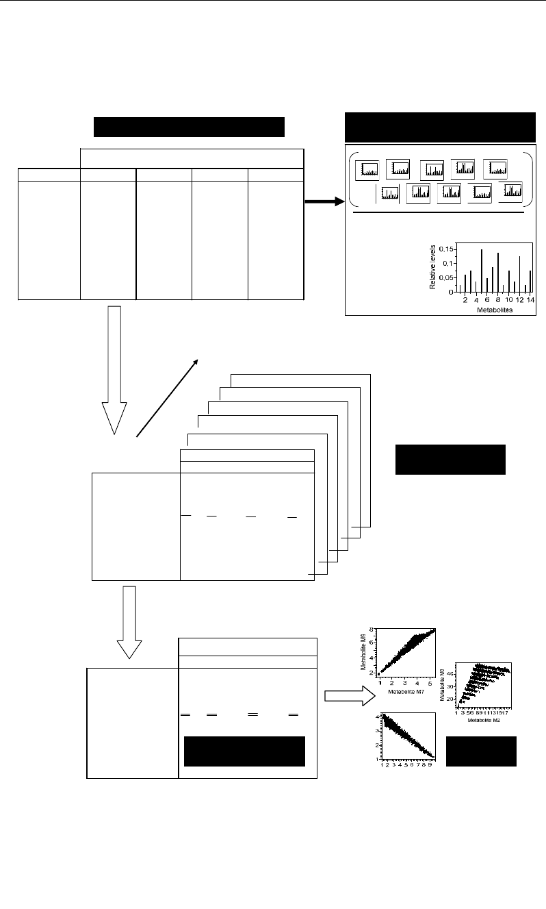
Figure 14. Metabolomic approach based on iterative Scheffe mixture design and leading to extract a set

of smoothed profiles representing a backbone of metabolic system from combinations of observed

profiles belonging to different patterns.

Nabil Semmar 18

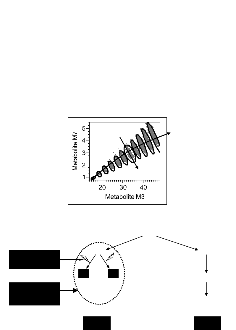
Figure 15a shows a relationship between two metabolites which is locally negative and

globally positive. In terms of metabolic processes, this can concern two metabolites which are

systematically competitive for a same precursor (negative local correlation) but which belong

to a same metabolic pathway leading them to compete together against other competitive

pathways (Fig 15b) (other metabolic trends) (Semmar et al., 2007).

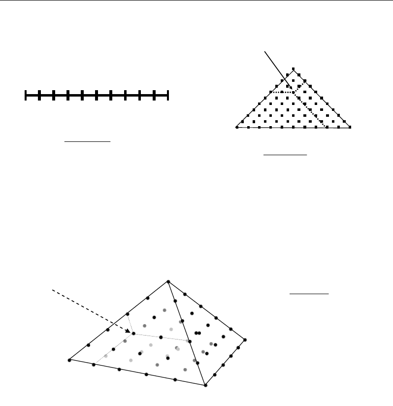
Figure 15a shows that the cloud of points has the fingerprints of a triangular shape. This

is due to the fact that the set of all the combinations of Scheffe matrix are contained within a

simplex network with a vertices number equal to the number q of components to combine

(e.g. q metabolic trends to combine) (Figure 16) (Eide I, 1996; Pattarino et al., 1993;

Nyieredy et al., 1985; Glajch et al., 1982; Semmar, 2010). Iterations of the mixture design

result in compressions and inclinations of the simplex space at degrees and under directions

depending on the different relationships between metabolites.

Negative local correlation

Positive global

correlation

M1

(a)

M2

M3

M10

M11

M12

M7

(b)

Metabolite

Metabolic

pathway I

Metabolic

pathway II

Global support of

metabolic pathway I

against pathway II

Local competition

for a same precursor

M2

Figure 15. (a) Illustration of a correlation locally negative and globally positive; (b) Possible metabolic

factor generating such scale dependent correlation, e.g. metabolites M3 and M7 compete each other in

metabolic pathway I (negative local correlation) but sustain their common pathway I against the

competitive pathway II (positive global correlation).

Correlations - and Distances - Based Approaches to Static Analysis… 19

(5, 0, 0, 0)

(4, 1, 0, 0)

(3, 2, 0, 0)

(2, 3, 0, 0)

(1, 4, 0, 0)

(0, 5, 0, 0)

(0, 4, 1, 0)

(0, 3, 2, 0)

(0, 2, 3, 0)

(0, 1, 4, 0)

(0, 0, 5, 0)

(0, 0, 4, 1)

(0, 0, 3, 2)

(0, 0, 2, 3)

(0, 0, 1, 4)

(0, 0, 0, 5)

(1, 0, 0, 4)

(2, 0, 0, 3)

(3, 0, 0, 2)

(4, 0, 0, 1)

(2, 0, 1,2)

56

!5)!14(

)!145(

=

−

+

mixtures

6, 2, 2

X

1

X

2

X

3

X

1

X

2

0 1 2 3

4 5 6 7 8

9 10

10 9 8 7 6 5 4 3 2 1

0

11

)!10()!12(

)!1210(

=

−

−+

=N

66

)!10()!13(

)!1310(

=

−

+

=N

(a) q=2, n=10 (b) q=3, n=10

(c) q=4, n=5

10, 0, 0

6, 4, 0

8, 0, 2

0, 2, 8

0, 10, 0 0, 0, 10

Figure 16. Different simplex representing different Scheffe mixture designs according to the number q

of components to combine and the number n of elements representing the q components in each

mixture.

IV. Metabolomic Approaches Based on Distance and Correlation

Matrices

The variability of a metabolomic dataset (n rows × p columns) can be analysed under

three aspects, viz. along rows, along columns, as well as through associations between rows

and columns (Figure 17) (Lindon et al. 2007; Sumner et al., 2003):

Column analysis focuses on the relationships between variables (metabolites) in order to

quantify and to fit the links between them. Such goals are provided by correlation analysis.

Row analysis tends to screen the similarities and differences between individuals (e.g.

metabolic profiles). This helps to classify the individuals into homogeneous groups that can

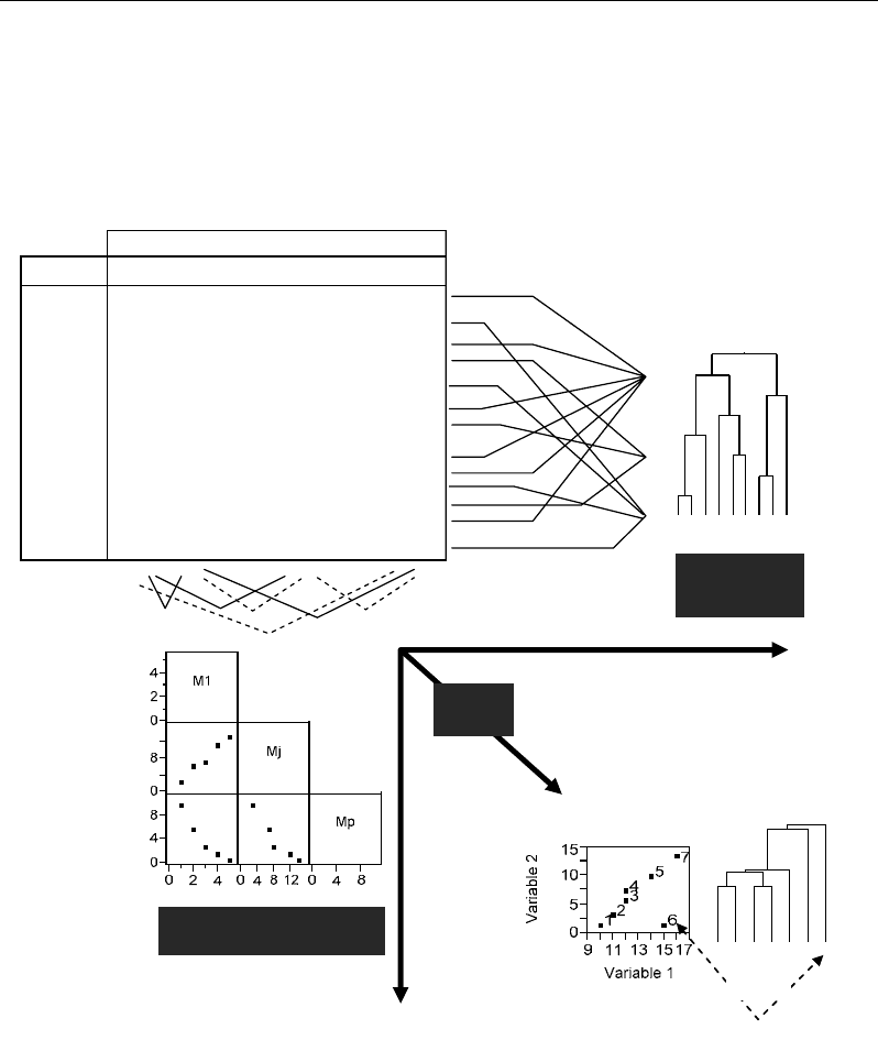
Nabil Semmar 20

be interpreted in terms of polymorphism poles within the studied population. Such fine

segmentation of the dataset (population) can be reliably performed by means of cluster

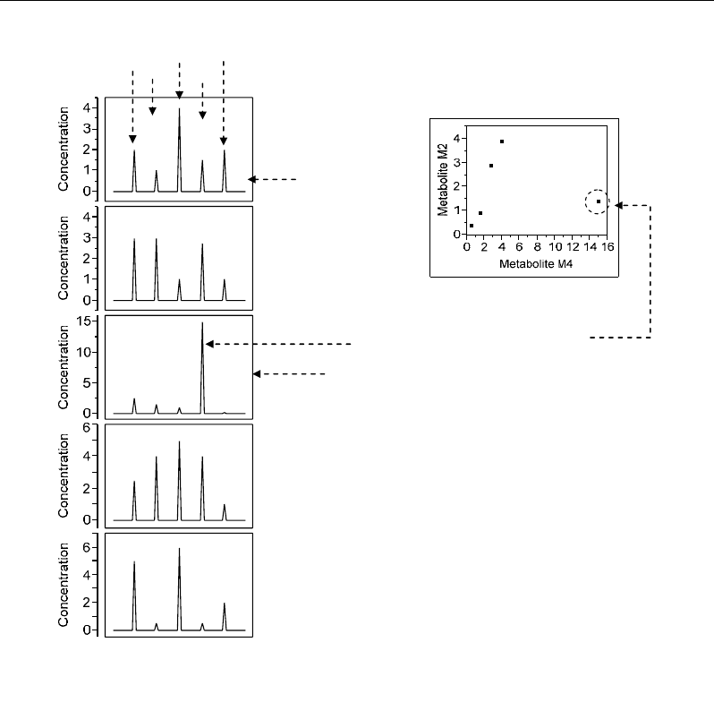
analysis. By considering both the rows and columns, extreme, atypical or original

associations between individuals and variables can be identified in the dataset. This leads to

analyse the heterogeneity or diversity degrees within the dataset and can be performed by

different outlier diagnostic approaches (Figure 18).

Cluster

Analysis

Correlation Analysis

Row-column

associations

1 2 3 4 5 7 6

Outlier

Metabolites

Profiles

M

1

M

2

…

M

j

…

M

p

1 C

11

C

12

…C

1j

…C

1p

2

C

21

C

22

…C

2j

…C

2p

: ………………

:

………………

i

C

i1

C

i2

…C

ij

…C

ip

: ………………

:

………………

n

C

n1

C

n2

…C

nj

…C

np

Row Analysis

Column

Analysis

Outlier

Analysis

Figure 17. Different statistical approaches applied in metabolomics corresponding to horizontal or

vertical data analysis.

Correlations - and Distances - Based Approaches to Static Analysis… 21

Atypical profile

Atypical metabolite concentration

Five Variables (Five columns)

One profile

(One row)

M1 M2 M3 M4 M5

Metabolites

Figure 18. Simple illustration of identification of atypical profiles and concentration values based on

profile (row) and variable (column) analyses, respectively.

IV.1. Correlation Based Approaches

Relationships between variables are subjected to correlation analysis which takes into

account the dispersion, global inclination and shape of data. Correlation analysis leads to

quantify the reciprocal effect of two variables each on the other. For that, different statistical

parameters are calculated, viz. correlation coefficients, confidence ranges, slopes, etc.

Correlation coefficient quantifies the monotony degree between variables, but it provides no

information on the kind of their relationship. Correlation coefficient gives also qualitative

information on the direction or inclination of the dataset through its sign: positive and

negative signs indicate increasing and decreasing trends, respectively. The inclination of the

cloud of points representing the dataset is quantified by the slope of the statistical model used

to describe the data variability. The model is defined by an equation which is used to fit well

the shape of the cloud of points. The most commonly used model is the linear model

Nabil Semmar 22

represented by the equation y=ax+b. Several other models can be used according to the shape

of cloud of points (y vs x), viz. logarithmic (y=Ln(x)), square root (y=√x), inverse (y=1/x),

exponential (y=e

x

). These models are also applied in order to bring data linearization leading

to benefit from computation and simplicity advantages of the linear model.

IV.1.1. Graphical Identification of Correlation Models

The first step in correlation analysis consists in visualising the bivariate data by means of

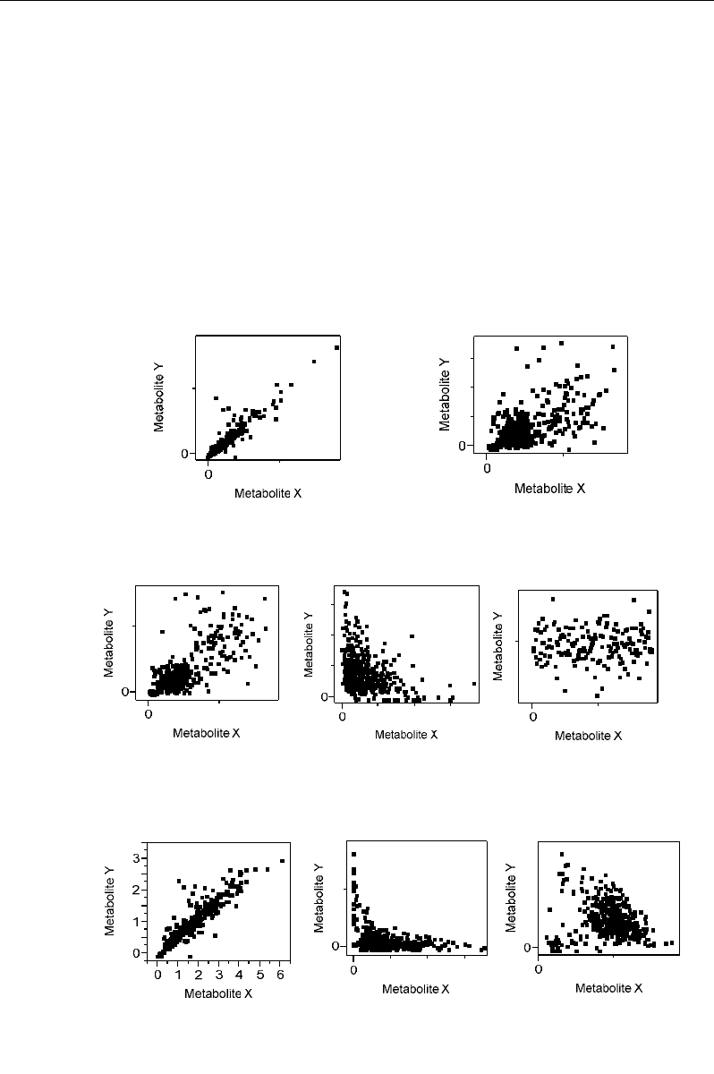
naïve scatter plots. One obtains clouds of points from which the relationships between

variables (metabolites) can be described on the basis of their dispersions, inclinations and

shapes (Figure 19).

Precise relationship

Dispersed relationship

Positive relationship

Dispersion

Inclination

Negative relationship

Linear relationship

Shape

Curvilinear relationship

Non-linear relationship

(e.g. scale dependent)

(a)

(b)

(c)

(d)

(f) (g) (h)

(e)

Not si

g

nificant

relationship

Figure 19. Different scatter plots showing different characteristics (dispersion, inclination, shape) from

which statistical tools can be appropriately used to quantify and to fit relationships between variables

(metabolites).

Correlations - and Distances - Based Approaches to Static Analysis… 23

For thin or few dispersed clouds of points (Figure 19a, f), relationships between variables

can be quantified by means of Pearson correlation coefficient. In the case of more dispersed

data (Figure 19b, c, h), Spearman correlation coefficient can be used as robust statistic to

detect trends between variables (metabolites). Positive (Figure 19a-c, f) and negative (Figure

19d, g) relationships will be indicated by positive and negative correlation coefficients,

respectively.

Pearson correlation is sensitive to the non linearity of data (Figure 19d, g, h). In the case

of curvilinear relationships, the use of Pearson coefficient can find application after data

linearization using an appropriate transformation. Appropriate transformations provide

symmetrical distributions (close to normal) of the data by reducing their dispersion,

asymmetry and bias effects of isolated (extreme) points (Zar, 1999). Such transformations can

be applied either on only one or on both variables of the pair (X, Y).

Moreover, such transformations are applied to stabilize the variances between several

groups of the dataset, i.e. in the case of heteroscedastic data (non comparable variances

between groups). Therefore, the resulting homoscedasticity will make possible the application

of linear model.

IV.1.2. Data Transformation to Application of Linear Model

From a graphical visualisation, a curvilinear cloud of points (Y vs X) can be transformed

into linear form by using an appropriate formula (Zar, 1999, Legendre and Legendre, 2000).

Such a formula depends on the shape, intensity of curvature and number of inflexion point(s)

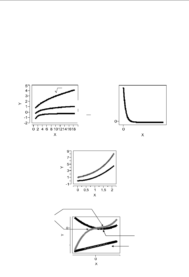
of the cloud of points Y vs X (Figure 20).

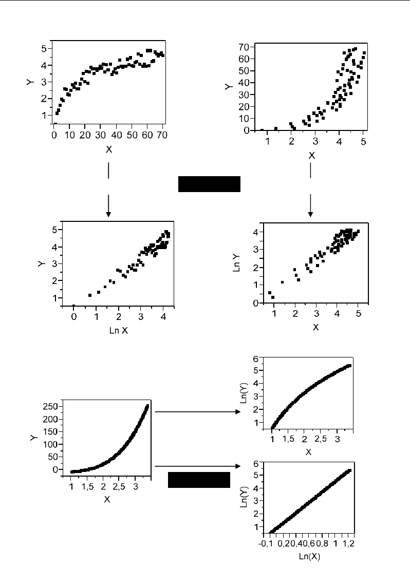
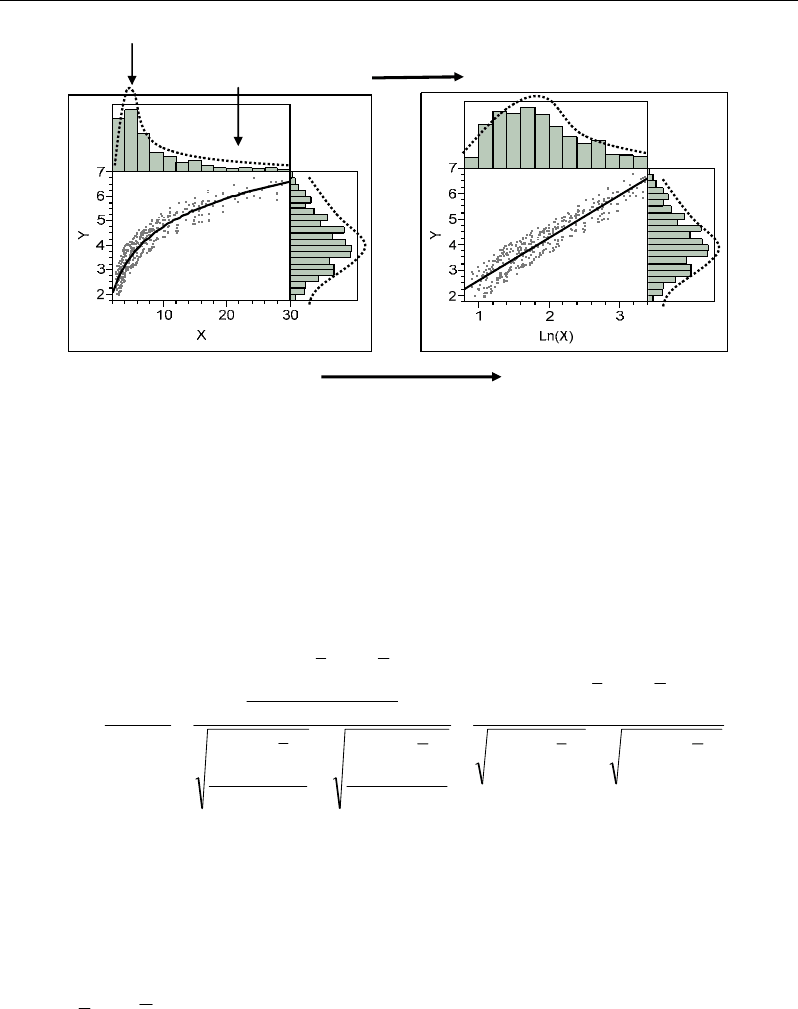
Logarithmic transformations are appropriate to linearize curvature showing slow (i) or

accelerated (ii) variations of Y vs X after an inflection (Figure 21). In the first case (i) (Figure

21a), linearization is obtained from Y vs Ln(X); in the second case (ii) (Figure 21b),

linearization is obtained from Ln(Y) vs X. More precisely, the fonction Y = a e

bX

is linearized

by taking the log of Y to give a straight-line equation with intercept Ln(a) and slope b, i.e.

ln(Y) = ln(a) + bX. In the case where Y and X are linked by a power function Y=a(X)

c

, such

non-linear relationship can be linearized by taking the logarithms of both X and Y, giving

linear equation ln(Y) = Ln(a) + c ln(X) (Figure 21c). In general, from a curvilinear cloud of

points, the appropriate model can be identified from the transformation by which the curve

becomes aligned (Figure 21).

Taking into account the distribution of each variable, logarithmic transformation can be

expected for a right asymmetric distribution, i.e. having a mode located at the left (a majority

of low values). Therefore, logarithmic transformation results in more symmetrical

distribution, i.e. a distribution which closer to normality conditions leading a possible

application of the linear model (Figure 22).

Square root transformation can be applied to linearize parabolic cloud of points.

Moreover, the square root can be preferred to the logarithm transformation (more generally

used) in the case of small dataset (few number of observations). Graphically, models

requiring square root transformation have more soft curvature than those requiring

logarithmic transformation (Figure 20a).

Clouds of points can be also linearized by means of polynomial transformations. This is

generally applied in the case where different inflection points are observed. Therefore, clouds

with k inflexion points can be fitted by means of polynomes with degree k+1 (Figure 20d).

Nabil Semmar 24

IV.1.3. Correlation Coefficient Computation

The correlation concept is used to measure the dependency degree between two variables

(metabolites). Such dependency degree between variables is quantified by a correlation

coefficient which can be characterised by two aspects: its absolute value and its sign.

Absolute value of correlation coefficient varies between 0 and 1; higher value indicates a

stronger dependency degree between the variables. All the same, small correlation values can

be statistically significant because of a great number of points confirming it. This can be

observed in large dataset containing many repeated experimental measurements. On the other

hand, some high correlations can be not significant because they were calculated on few data.

XY =

)(

10

XLogY

=

X

Y

1

−=

X

eY

−

=

1 inflexion point

⇒ Y=f(X²)

0 inflexion point

⇒ Y=f(X) =aX+b

2 inflexion points

⇒ Y=f(X

3

)

X

eY =

2

X

Y

=

(c)

(a) (b)

(d)

Y

Figure 20. Linearization of different curvilinear relationships by using appropriate data transformations.

Correlations - and Distances - Based Approaches to Static Analysis… 25

Ln Y=f(X)

Y=f(Ln X)

(a) (b)

Ln(Y) vs X

Ln(Y) vs Ln(X)

(c)

Linearization

Figure 21. Applications of logarithmic transformations for data linearization.

Nabil Semmar 26

Mode at the left

Asymmetrical at right

Less asymmetrical

(tends to symmetry)

Ln(X)

Curvilinear model

Linear model

X → Ln(X)

Figure 22. Logarithmic transformation leading to attenuate right asymmetric distribution to become

close to normality conditions allowing linear model application.

IV.1.3.1. Pearson Correlation Computation

The Pearson correlation coefficient (r) between two variables x and y is calculated by

using the following formula tacking into account their variances and covariance:

2

11

2

1

2

11

2

1

)(.)(

))((

1

)(

.

1

)(

1

))((

.

∑∑

∑

∑∑

∑

==

=

==

=

−−

=

−

−−

==

n

i

n

i

n

i

ii

n

i

n

i

n

i

ii

yx

xy

yyxx

n

yy

n

xx

n

yyxx

SS

C

r

where:

C

xy

is the covariance of the variables x and y

S

x

and S

y

: are the standard deviations of x and y

x

i

and y

i

are measured values (concentration values) of the variables x and y,

respectively, in individual i

x

and

y

are the means of the variables x and y, respectively.

n is the number of paired values (x

i

, y

i

) (total number of individuals or rows i in the

dataset).

Let’s give a numerical example to illustrate the calculus of Pearson correlation (Figure

23). Suppose we have a metabolic dataset (10 rows × 4 columns) describing 10 profiles by the

concentrations of 4 metabolites:

Knapp J.S., Cabrera W.L. Metabolomics: Metabolites, Metabonomics, and Analytical Technologies

Подождите немного. Документ загружается.