Hungerford T.W., Shaw D.J. Contemporary Precalculus: A Graphing Approach
Подождите немного. Документ загружается.

9. $366.67 at 12% and $733.33 at 6%
11. 2
2
3
qt 13. 60 mph 15. 44, 38.25
17. 65 mph 19. About 1.753 ft 21. 2 meters
23. About 132.7 ft
25. Red Riding Hood, 54 mph; wolf, 48 mph
27. 2.234 in. 2.234 in. 29. 4.658 in. 31. 8.02 in.
33. 11.47 ft or 29.91 ft 35. 6.205 miles
37. 157.6 mph 39. 2.2 4.4 4 ft
Section 2.4, page 118
1. (1, 8) 3. (1.142855, 2.0625)
5. (.3409, .0003222)
7. (a) (1, 4) (b) (1, 4) and (2, 4) (c) (3, 20)
9. 52.86 mph 11. 21 ft
13. 450 ft 900 ft 15. $8800
17. 34.2 cm 34.2 cm 17.1 cm
19. (a) 4.4267 by 4.4267 in. (b) 10/3 by 10/3 in.
21. (a) Approximately 206
(b) Approximately 269; approximately $577
23. (a) 600 (b) 958
25. x 9.306; area 220.18 ft
2
27. Approximately (1.871, 1.5) 29. 12 times
Section 2.5, page 128
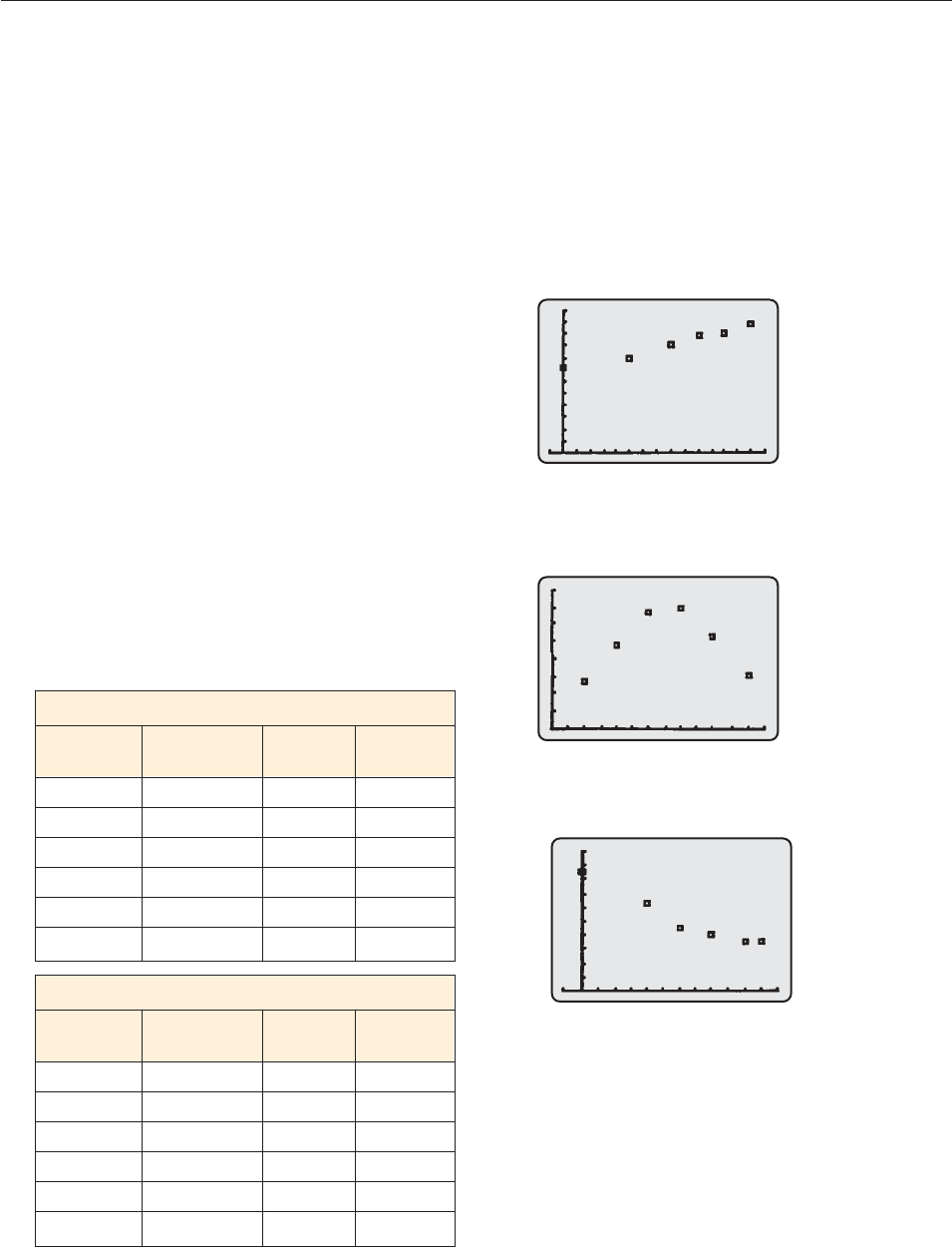
1.
The model y .5x 1.5 is better.
976 ANSWERS
3. (a) Data points are (0, 171.3), (2, 179.8), (4, 188), (6, 201.5).
For y 4.9x 170, the residuals are 1.3, 0, 1.6, 2.1;
their sum is 1.8. For y 5x 171, the residuals are .3,
1.2, 3, .5; their sum is 3.4.
(b) The sum is 8.66 for y 4.9x 170 and 10.78 for y
5x 171.
(c) The first model is a better fit.
5. The sum is 1.9055, whereas the sums for the other two mod-
els are 2.8 and 2.75.
7. Negative 9. Negative
11.
(a) The data appears linear.
(b) Positive correlation
13.
(a) The data is not linear.
15.
(a) The data appears linear.
(b) Negative correlation
17. (a) y 14.9x 2822
(b) 5057, 6994, 9080; the estimates are quite close to the
actual values.
(c) 6323.5; 6500
19. (a) (6, 1.8), (7, 2.3), (8, 2.5), (9, 3.1), (10, 3.9),
(11, 3.8), (12, 4), (13, 4.4), (14, 4.8), (15, 5.1)
(b) y .3594x .2036
(c) About $6.98 billion
1,000,000
5
0
60
80
0
0
13
12,000
0
0
15
MODEL: y x
Squared
Data Point Model Point Residual Residual
(1, 2) (1, 1) 1 1
(2, 2) (2, 2) 0 0
(3, 3) (3, 3) 0 0
(4, 3) (4, 4) 11
(5, 5) (5, 5) 0 0
Sum: 0 Sum: 2
MODEL: y .5x 1.5
Squared
Data Point Model Point Residual Residual
(1, 2) (1, 2) 0 0
(2, 2) (2, 2.5) 0.5 0.25
(3, 3) (3, 3) 0 0
(4, 3) (4, 3.5) 0.5 0.25
(5, 5) (5, 4) 1 1
Sum: 0 Sum: 1.5
21. (a) y 9.9429x 600.8095 and
y 20.2286x 900.4286
(b) Earnings are increasing at the approximate rate of
$9.63, $16.29, $9.94, and $20.23 per week respectively.
23. (a) y .2179x 52.2805
(b) y .1447x 65.4246
(c) Yes; in 2079
25. (a) y .03119x .5635
(b) About .938 billion; about 1.06 billion
Chapter 2 Review, page 132
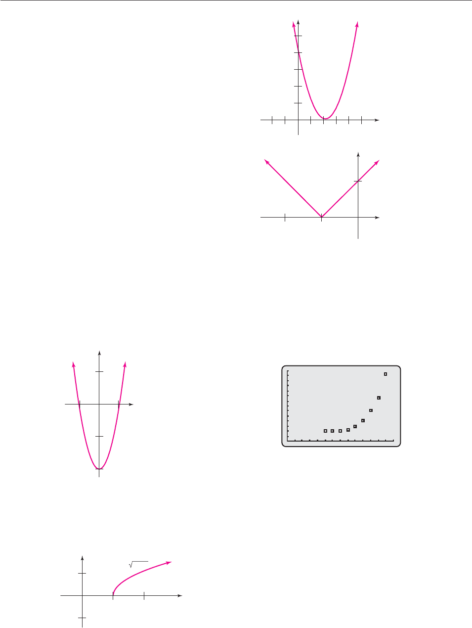
1. (a) a, d
(b) b, c do not show peaks and valleys near the origin; e
crowds the graph onto the y-axis.
(c) a or 4 x 6 and 10 y 10
3. (a) None of them
(b) a, b, d do not show any peaks or valleys; c does not show
the valleys; e shows only one point on the graph (which
can’t be distinguished because it’s on the y-axis).
(c) 7 x 11 and 1000 y 500
5. (a) b, c
(b) a shows no peaks or valleys; d is too crowded horizon-
tally; e shows only one point.
(c) 10 x 10 and 150 y 150
7. As x moves left or right from the origin, x
2
grows larger and
larger, and hence so does x
2
10. Therefore, the graph always
rises as it moves away from the y-axis and is complete.
9. Note that y is defined only when x 5 (why?). Also, x 5
grows larger as x gets larger (that is, as you move to the right)
and hence the same is true of x 5
. Therefore, the graph
always rises as you move to the right and is complete.
510
y = x − 5
–2
2
x
y
3
y = x
2
− 10
–3
–5
–10
5
x
y
ANSWERS 977
11.
13.
15. x 2.7644 17. x 3.2678
19. x 3.2843 21. x 1.6511
23. Gold,
1
3
1
oz; silver,
1
8
1
oz
25. 2
2
9
hrs 27. 9.6 ft
29. 4 ft 31. 25
33. 20 yd by 30 yd (interior fence is 20 yd)
35. x 3
1.732
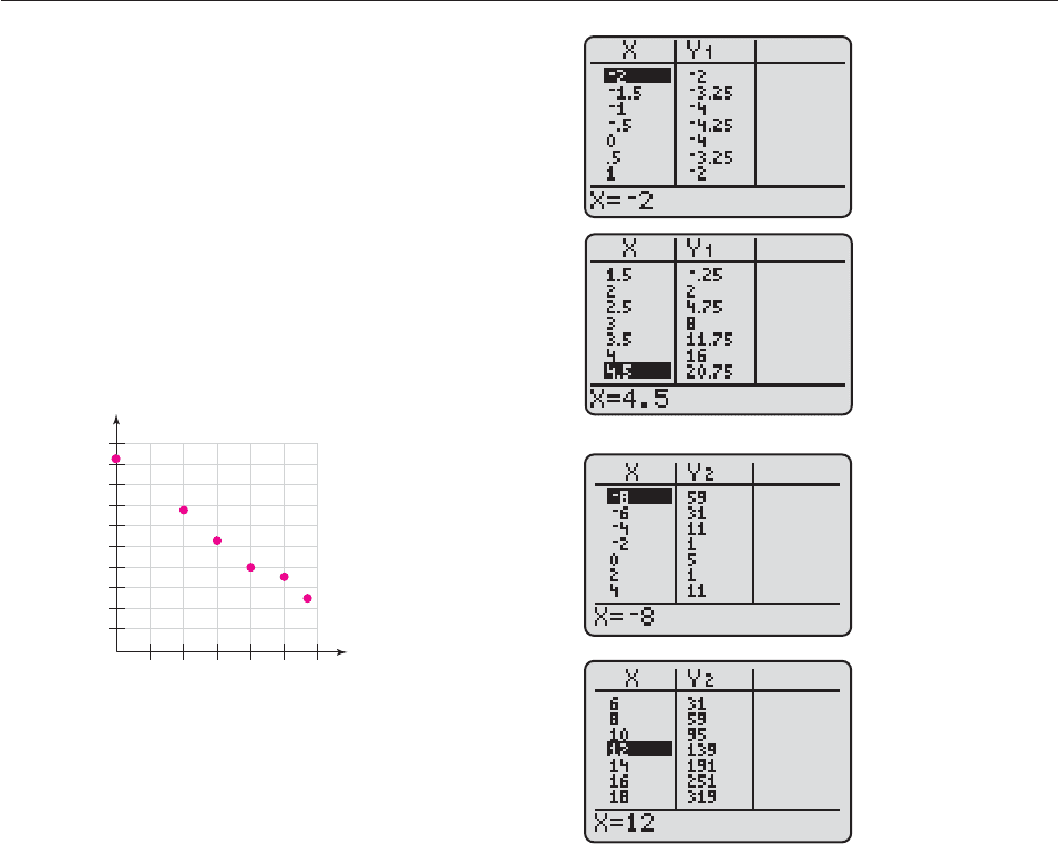
37. (a)
(b) Nonlinear
39. (a) y 1.5868x .2473
(b) 89 and 108 years respectively (c) About 2.5 ft
41. (a) y 14.8998x 59.0163
(b) $193.1 billion in 1999; $297.4 billion in 2008
(c) in 2011
Chapter 2 Test, page 135
1. The standard viewing window clearly shows the parts of the
graph near the origin. To see the rest of the graph a larger win-
dow is needed, such as 4 x 14 and 212 y 10.
2. x 17 3. (8.1510, 95.8884)
4. (a) 5 (b) any k such that k 4.43 or k 4.43
0
70
0
140
−5
x
y
−10
5
y =⏐x + 5⏐
36−6 −391512
x
y
10
20
30
40
50
y = x
2
− 13x + 43
5. 12 x 12 and 8 y 8 on a standard screen (such
as TI-84); on a wide-screen calculator, 6 y 6 pro-
duces an approximately square window.
6. x 2, but x 2 is not a solution (why?).
7. (a) 0 x 48 and 0 y 30
(b) t 7.937 hours; 26.457 mg per liter
8. x 1.3865 or .4258 9. (35 x)(40 x) 785
10. 8.347 in by 7.4 in 11. 1.14 qt
12. (a) (1, 1.1) (b) (2, 1.1)
13. 27 cm by 28 cm by 29 cm
14. About 1942 15. 2.3 ft by 4.6 ft by 4 ft high
16. (a) 2.937 in by 2.937 in (b) 2 in by 2 in
17. (a)
(b) Yes; negative (c) y 11.823x 912.576
18. (a) Residuals: .4, .5, .3, .8; sum of residuals; 1; sum of
squares of residuals: 1.14
(b) Residuals: .5, 1.8, 1.2, .9; sum of residuals;
4.4; sum of squares of residuals: 5.74
(c) The model in part (a) is the better fit.
19. (a) y .3272x 5.0259
(b) About 7.6 million barrels per day in 2008 and about
10.9 million barrels per day in 2018
20. (a) y 19.2286x 206.0952
(b) About 340,700 vehicles
(c) About 19,200 cars per year
Chapter 3
Section 3.1, page 148
1. This is a function because, for every input there is a unique
output.
3. This could not be a table of values of a function, because
two output values are associated with the input 5.
5. 6 7. 2 9. 17
11. This defines y as a function of x.
13. This defines x as a function of y.
15. This defines both y as a function of x and x as a function of y.
17. Neither
500
10 20 30 40 50 60
300
100
900
1000
700
400
200
800
600
x
y
978 ANSWERS
19.
21.
23. $8.40, $31.69, $693.75, $521.25, $262.50, $2150.17
25. A function may assign the same output to many different
input.
27. Postage is a function of weight, but weight is not a function
of postage; for example, all letters less than one ounce use
the same postage amount.
29. This could not be the rule of a function, since, for example,
it would assign two numbers (2 and 2) to the input 4.
31. (a) Jan. 2000, 8
1
⁄2%. Jan. 2001, 9
1
⁄2%. Mid-2005, 6%.
(b) After Jan. 2002 until Dec. 2004.
(c) The prime rate is a function of time, but time is not a
function of the prime rate.
33. (a) A x
2
(b) A
d
2
2
35. S 10pr
2
37. C 125x 26,000
39. (a) y 2.3107x 20.0821 (b) $40.9 million
41. Output for 2 is 2. The output for 1 is 0. The output for
0 is approximately 1
1
⁄4 and the output for 1 is approximately
2
3
⁄4.
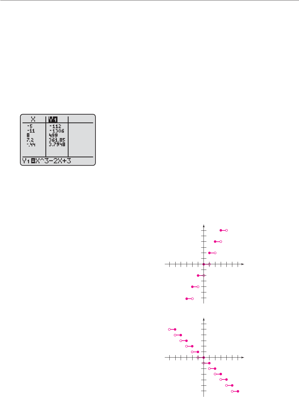
43. Output for 2 is 1. The output for 0 is 3. The output for
1 is 2.
The output for 2.5 is 1.
The output for 1.5 is 0.
45. Output for 2 is 1. The output for 1 is 2.9. The output
for 0 is 1. The output for
1
⁄2 is 1. The output for 1 is 1
1
⁄2.
47. (a) x 0
(b) 1 y 1 where y cos(ln x)
49. (a) For a nonnegative number, the part of the number to the
left of the decimal point (the integer part) is the closest
integer to the left of the number on the number line.
(b) the negative integers.
(c) negative numbers that are not integers.
51. (a)
(b) 10
3
2(10) 3 983
Section 3.2, page 158
1. (a) .8 (b) .75 (c) .4 (d) .125 (e) 0
3. 3
1 5. 2
3
2
1
7. 4 9. 17.75
11. p
2
2p 3
p
1
1
13. (a k)
2
a
1
k
2
15. x
2
1
x
2 17. x
2
6x 11
x
1
3
19. s
2
2s 21. t
2
1
23. 11 7 25. 1
27. 3 29. 1 2x h
31.
x
1
h
x
33. 2x h
35. (a) f(a) a
2
, f(b) b
2
, f(a b) (a b)
2
a
2
2ab
b
2
, so (a b)
2
a
2
b
2
, that is, f(a b) f(a) f(b)
(b) f(a) 3a, f(b) 3b, f (a b) 3(a b)
3a 3b f(a) f (b).
(c) f(a) 5, f(b) 5, f(a b) 5, f(a b) f(a) f(b)
37. c 2
39. (a) 3 x 4 (b) 2 y 3 (c) 2
(d) 1/2 (e) 1 (f) 1
41. x
43. (a) x 20 (b) 3 (c) 1 (d) 1 (e) 2
45. all real numbers 47. all real numbers
49. x 0 51. all real numbers except 0
ANSWERS 979
53. all real numbers
55. all real numbers except 3 and 2
57. 6 x 12
59. Many examples including f(x) x
2
and g(x) x
4
.
61. Many examples including g(x) x
3
.
63. 3/2, 4 65.
3
2
21
67. f(x) 8 3x
2
69. P(x) .7x 1800
71. (a) 38 .72y
(b) 2 .72x
73. d
75. (a) y 108 4x
(b) V x
2
(108 4x) 108x
2
4x
3
77. C 2t
2
2
t
0
79. (a) f(x) 18.3x 244.4
(b) g(8) 391, g(11) 446. These are not that accurate,
but in the right ballpark
(c) g(10) 427
(d) g(21) 629
Section 3.3, page 171
1. Yes, f(3) 0 3. No
5.
7.
1
1
x
y
1
1
x
y
0 t 2
t 2
55t
20 45t
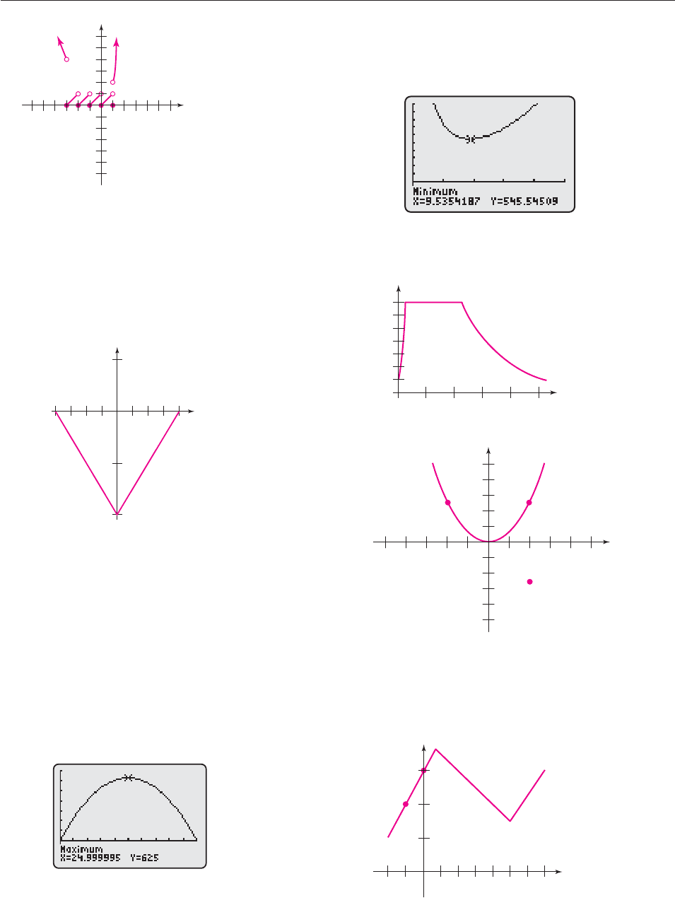
9.
11.
The graph fails the vertical line test; hence, it cannot be the
graph of a function. For example, x 3 corresponds to both
5 and 9.
13. [3, 5] 15. [3, 3) 17. 3.5
19. 4.5 21. 1 and 5
23. (a) h(x)
(b)
25. If 0 x 2, then x 2 0. So by the definition of ab-
solute value, x 2 (x 2) x 2. Also, since
x 0, x x. Hence, f(x) x x 2 x x 2 2
for all x between 0 and 2.
27. Maxima at (4, 0), minimum at (0, 4)
29. Maximum at (1, 3), minimum at (1, 1)
31. None
33. Decreasing when x 5.8 and x .46, increasing when
5.8 x .46
35. Only decreasing in (, 0) U (0, )
37. (a) 2x 2z 100
(b) A(x) x(50 x)
(c)
x 25 inches, z 25 inches
−200
50
700
0
1
1
1
2
x
y
23434 2 1
x 0
x 0
2
x
2
2
x
2
1
4
x
y
980 ANSWERS
39. (a) S 2x
2
4xh
(b) x
2
h 867
(c) S 2x
2
34
x
68
(d)
x 9.5354 inches, h 9.5354 inches
41. (a) (iv) (b) (i) (c) (v) (d) (iii) (e) (ii)
43.
Domain is x 0, range is 50 y 350.
45.
47.
(a) 9%, 16%, 8%
(b) Lowest: 2003. Highest: 1990
(c) 1980–1983; steepness of curve
49. (a) False
(b) False
(c) False
51.
2 1
1
2
3
1234567
x
y
k
k
(k, −f(k))
(k, f(k))
f(k)
(−k, f(−k))
20 40 60 80 100
350
300
250
200
150
50
100
y
x
−300
25
1000
0
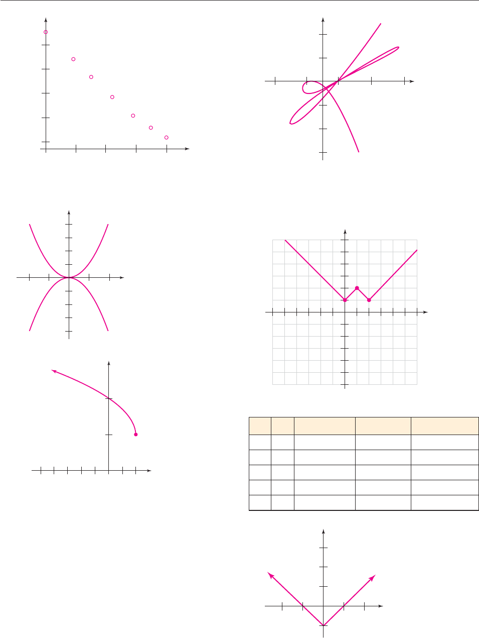
53. (a)
(b) y .545x 41.8 (c) 27.7%, 15.7% (d) 2014
(e) It will disappear completely in 2042 according to this
model.
55.
57. (a) (, 4] (b) [2, )
(c)
59. After 15 minutes she took a break then picked up her pace
for 10 minutes. After 30 minutes she jogged back home at a
constant rate for a total jog of 55 minutes.
Section 3.3.A, page 178
1. 6 x 44, 0 y 16
3. 2 x 32, 60 y 60
5. 16 x 2, 60 y 60
7. 50 x 50, 7 y 3, 7 t 3 (answers will vary)
9. 8 x 5, 5 y 5, 5 t 5 (answers will vary)
11. 10 x 7, 0 y 2, 0 t 2 (answers will vary)
420246810
x
2
4
y
4
3
2
1
4
3
2
1
y
2 1
12
x
x
10
20
25
30
40
35
20 30 400
y
ANSWERS 981
13.
It crosses itself 6 times
Section 3.4, page 186
1. H 3. F 5. K 7. C
9.
11.
13.
−4 −2
24
−2
2
4
6
x
y
x
y
224646
2
2
4
6
4
6
30
20
10
10
20
y
15 5
15 25
x
5
tf(t) g(t) f(t) 3 h(t) 4f(t) i(t) f(t 1) 2
2 3 0 20 Not possible
16 3 0 1
08 5 32 4
10 324 6
25 2 12 2
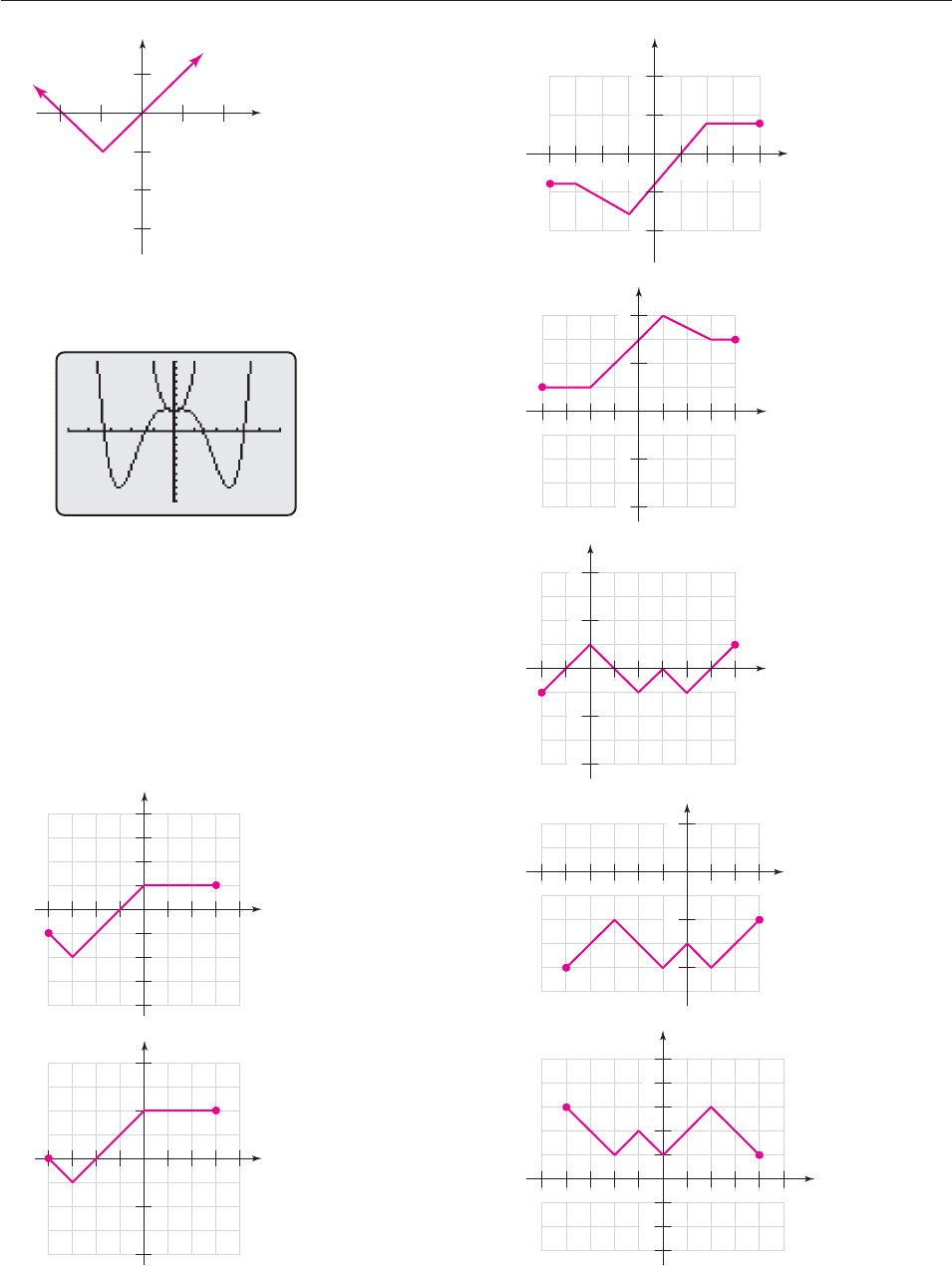
15.
17.
15 x 15 and 12 y 10
19. 5 x 7 and 10 y 10
21.
23.
Shift 2 units to the left then 5 units up.
25. Reflect across the x-axis, then stretch vertically by a factor
of 2, and then shift 10 units up.
27. g(x) x
2
x 2 29. f (x)
1
2
(x
3)
31. (a) g(x) x
2
2x 6
(b) difference quotient for f: 2x h; difference quotient for
g: 2x h 2
(c) 2x h 2 2(x 1) h d(x 1)
33.
35.
x
y
2 1323144
1
1
x
y
2 1323144
2
4
2
4
−10
10
−55
−4 −2
24
−2
−4
−6
2
x
y
982 ANSWERS
37.
39.
41.
43.
45.
−2
2
4
x
y
−2−3−4−5 −1
2
3 4 51
−2
2
−4
x
y
−6 −2−3−4−5 −1
2
31
−2
2
4
−4
x
y
−2 −1
26
3 4 51
−2
2
4
−4
x
y
−4 −2−3 −1
24
31
−4 −2−3 −1
231
−10
−5
5
10
4
x
y
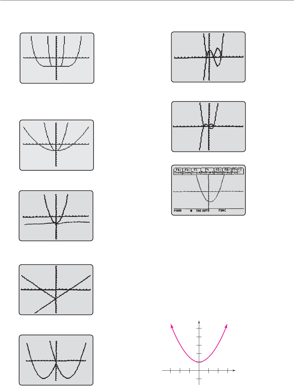
47. (a) The graph shifts 35 units up.
(b) The graph stretches in the y-direction.
49.
51.
The graph of f(cx), with c 1, is the graph of f(x)
contracted toward the y-axis by a factor of c.
53.
55.
57.
59.
−10
−10
10
10
−10
−10
10
10
−10
−10
10
10
−10
10
−10 10
−10
10
−10 10
ANSWERS 983
61. For x 0, f (x) and g(x) are the same. For x 0, g(x)
f(x).
63.
65.
67.
(a)
h(x) will look just like f(x), shifted 1000 units to the
right
(b) 990 x 1010, 10 y 10
(c) The problem is difficult because we have to include x
values that are 1000 units apart, which makes seeing
any details of the graphs impossible.
(d) g(x) should look like f(x), only stretched by a factor of
1000
(e) 10 x 10, 10000 y 10000. While we can
display both f and g, any window that shows g in detail
will not show f in detail.
Section 3.4.A, page 193
1.
Graph has y-axis symmetry
−1−2−3
231
−2
2
4
6
8
10
x
y
−10
−10
10
10
−10
−10
10
10
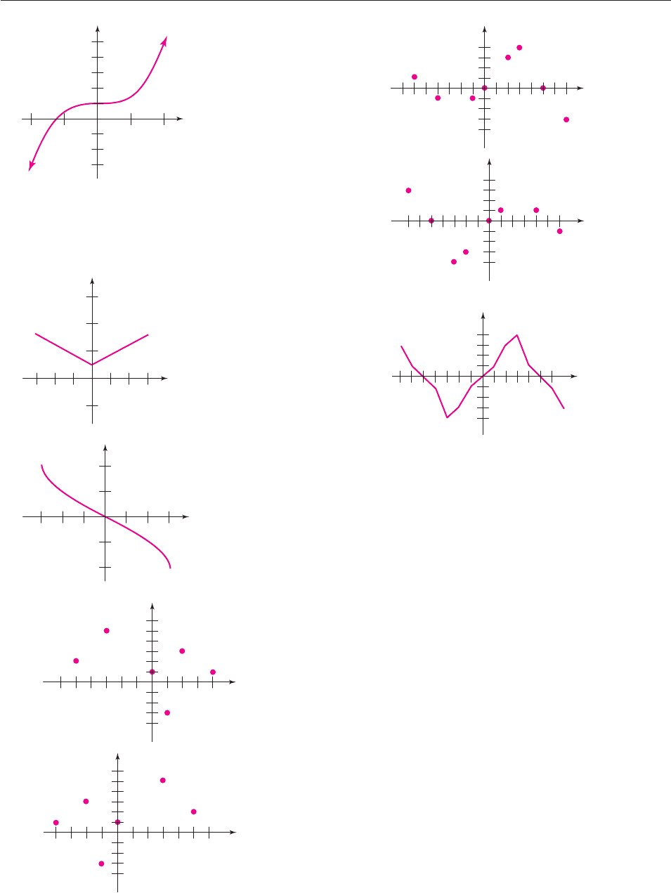
3.
5.
Odd 7. Even 9. Even
11. Odd 13. Even 15. Even
17. Yes 19. No 21. Origin
23. Origin 25. y-axis 27. None
29.
31.
33.
(a)
(b)
−3
36
−2
−4
2
6
4
x
y
−6 −3
3
−2
−4
2
6
4
x
y
−3 −2 −1
231
−2
−4
2
4
x
y
−2−3 −1
231
−2
2
4
6
x
y
−2 −1
21
−4
−6
−2
2
4
6
8
10
x
y
984 ANSWERS
35. (a)
(b)
(c) Many correct answers, including this one.
37. If replacing x by x does not change the graph and replac-
ing y by y does not change the graph, then doing both does
not change the graph. Thus, x-axis plus y-axis symmetry
guarantees origin symmetry. If replacing x by x does not
change the graph and replacing y by y does change the
graph, then doing both must change the graph. Thus, y-axis
symmetry and origin symmetry without x-axis symmetry is
impossible. The argument is analogous for x-axis and origin
symmetry.
39. (a) No because as the advertising budget increases, so do
the sales which is an increasing function which is not a
property of even functions.
(b) Yes, because as the advertising budget increases, so do
the sales which is an increasing function which is a
property of odd functions.
Section 3.5, page 202
1. x
3
3x 2; x
3
3x 2; x
3
3x 2
3. x
2
2x 5
1
x
;
1
x
x
2
2x 5; x
2
2x 5
1
x
5. 3x
4
2x
3
;
3x
x
3
2
;
3x
x
3
2
7. x
2
25,
x
x
5
5
,
x
x
5
5
9. All real numbers except 0; all real numbers except 0
11. 4/3 x 2; 4/3 x 2
−6 −3
36
−4
−2
4
2
x
y
−6 −336
−2
−4
2
4
x
y
−6 −336
−2
−4
2
4
x
y
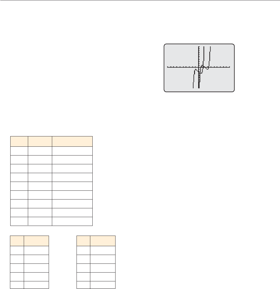
13. 0 15. 30
17. 49; 1; 8 19. 3; 3; 0
21. 3x
3
2, all real numbers; (3x 2)
3
, all real numbers
23.
2x
2
1
1
, all real numbers except
2
2
;
4
x
2
4
x
2
4
x
4x
1
, all
real numbers except 12
25. x
6
; x
9
27.
x
1
2
; x
29. ( f g)(x) f (g(x)) 9g(x) 8 9
x
9
8
8
x 8 8 x; (g f )(x) g( f (x))
f(x)
9
8
9x
9
8 8
9
9
x
x
31. ( f g)(x) f (g(x))
3
g(x)
2
3
(x 2
)
3
2
x 2 2 x; (g f )(x) g( f (x)) ( f (x) 2)
3
(
3
x
2 2)
3
(
3
x
)
3
x
33.
35. 37.
There may be correct answers to Exercises 39–44, other than
those given here.
39. Let g(x) x
2
2 and h(t)
3
t
. Then (h g)(x) h(g(x))
3
g(x)
3
x
2
2
.
41. Let g(x) 7x
3
10x 17 and f (t) t
7
. Then ( f g)(x)
f (g(x)) (7x
3
10x 17)
7
.
43. Let h(x) x
2
2x
k(t) t 1
45. Domain of f g : x 0 Domain of g f : x 0
47. Domain of f g : x 2 Domain of g f : x 10
ANSWERS 985
49. (a) 2x
6
5x
2
1
(b) 4x
6
20x
4
4x
3
25x
2
10x 1
(c) The answers are not the same. We conclude f(x
2
)
( f (x))
2
in general.
51.
Functions are not the same.
53. x
2
6x 10; 2x h 6
55.
2
x
;
x(x
2
h)
57. (a) about 1.22 10
4
square inches, about 2.5 10
6
square inches, about 1.36 10
7
square inches
(b) no, no, over a certain time period
59. (a) A
p
4
d
2
p
4
6
t
2
50
10
2
(b) about .7854 square inches, about 22.265 square inches
(c) about 11.4 weeks
61. V(t)
256
3
pt
3
, about 17,157 cm
3
63. s(t)
1
3
0t
65. f(x) x
67. (a) As the composition is applied you will stabilize at .1708
(b) yes.
(c) Now we wind up oscillating between .8873 and
.1127 (starting at either 0 or 1)
(d) We wind up cycling between four numbers this time.
Section 3.6, page 214
1. (a) 14 ft per sec
(b) 54 ft per sec
(c) 112 ft per sec
(d) 93.3 ft per sec
3. (a) 9954.5 million subscribers/year
(b) 19218.6 million subscribers/year
5. (a) Decreasing at 291,000 per year
(b) Increasing at 541,800 per year
(c) Increasing at 353,500 per year
(d) Increasing at 179,778 per year
(e) Fastest from 1985 to 1995, slowest from 2005 to 2014
7. (a) 29.18 (b) 51.8
(c) 24.08 (d) 33.5
(e) 1999 to 2001
−10
10
−10 10
xf(x) g(x) f ( f (x))
4 3 1
3 11/2
20 1
11/25/4
01 3/2
13/22
21 3/2
3 20
4 20
x (g f )(x)
14
22
35
44
54
x ( f f )(x)
11
23
33
45
51
