Hooke R.L. Principles of glacier mechanics

Подождите немного. Документ загружается.

Intercomparison of models 301

mean annual temperature and the Milankovitch cycles, or may be

calculated in another model, such as a global climate model (GCM).

If the output from an ice-sheet model is used as input for a time step in

a GCM, the output of which is then used for the next time step in the

ice-sheet model, the models are said to be coupled.

Validation

Once a model has been programmed and appears to be giving reasonable

results, it must be validated to ensure that there are no subtle errors

that affect the results signiﬁcantly but not so much as to make them

obviously unrealistic. A common way to initiate the validation process

is to set parameters in the model in such a way that the model duplicates

a situation for which there is an analytical solution. For example, if

∂θ/∂t, u, and Q are set to zero in Equation (11.12) and w is assumed

to be downward and to decrease linearly with depth, the model should

reproduce the Robin (1955) solution (Equation (6.24)). In ﬂow models,

the deformation of an inﬁnite slab of ice on a uniform slope (Equation

(10.42)) is a good choice. Of course, once these comparisons have been

made, there is still the question of whether coding of some of the terms

neglected in the test, such as u(∂θ/∂x)inEquation (11.12), is correct.

The modeler will have to be more imaginative to ﬁnd independent ways

to test these algorithms. One possibility is to compare the output of

similar models developed totally independently, as discussed next.

Intercomparison of models

Because of the large number of ice sheet models being developed, each

employing slightly different approaches and each subject to inadvertent

programming errors, a group of 16 modelers developed a set of tests

for comparison of models (Huybrechts et al., 1996;Payne et al., 2000).

One test, for example, utilizes a square domain, 1500 km on a side,

with grid points at 50 km spacing. Initially there is no ice sheet in the

domain. A radially symmetric mass balance pattern is speciﬁed as are the

ﬂow law constants n and B, and other relevant parameters such as ρ, g,

and κ. Because the speciﬁed mass balance pattern is radially symmetric

and constant with time, a model, when stepped through time, eventually

produces a steady-state circular ice sheet.

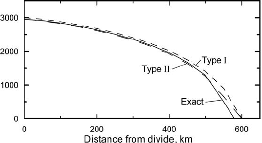
An intercomparison of twelve ﬁnite-difference models done using

this test found that most of the differences among them were inconse-

quential. The only signiﬁcant difference was between so-called Type I

and Type II models. Type I models used a mass ﬂux parameterization that

conserves mass but requires short time steps to achieve stability. Type II

302 Numerical modeling

Elvevation, m

Figure 11.5. Ice sheet

proﬁles calculated using Type I

and II ﬁnite-difference models

compared with an exact

solution. (After Huybrechts

et al., 1996, Figure 5a. Used

with permission of the authors

and the International

Glaciological Society.)

models do not conserve mass, but have the advantage of allowing longer

time steps. The means and standard deviations of the thicknesses of the

model ice sheets at the divide were 2997 ± 7.4 m and 2959 ± 1.3 m

for Types I and II models, respectively. An exact solution, obtained by

integrating the mass balance function analytically, produced an ice sheet

that was 20 km smaller in radius, and consequently somewhat thinner,

but a model with a 50 km grid spacing cannot get closer. Surface proﬁles

predicted by the two model types are compared with each other and with

the exact solution in Figure 11.5.

The tests developed by these modelers, normally referred to as the

EISMINT (European Ice Sheet Modeling INiTiative) benchmark tests,

are an invaluable tool. Both new models that are developed and existing

models that are being reﬁned can be tested against these benchmarks to

expose errors in reasoning or programming.

Sensitivity testing and tuning

Because the parameters used to the deﬁne boundary conditions, initial

conditions, and forcing are rarely known precisely, modelers normally

test the sensitivity of their models by varying these parameters within

reasonable limits. Suppose, for example, that the most likely temperature

boundary condition for a particular model is −5

◦

C, and suppose further

that it is unlikely that the correct boundary temperature is lower than

−7

◦

Corhigher than −1

◦

C. The modeler then might run the model

with all three temperatures to see if the conclusions changed when the

extreme temperatures are used. If the conclusions are unchanged, the

model is said to be robust against a reasonable range of temperature

boundary conditions. Such tests are called sensitivity tests.

Coupling thermal and mechanical models 303

If there are N parameters that are only known approximately and if

the maximum likely, minimum likely, and most probable values of all

combinations of the parameters is to be tested, the total number of tests

will be 3

.IfN > 3, such a task becomes daunting.

In a similar vein, models are often tuned so that they reproduce

observed characteristics of a glacier. For example, in the model of the

Barnes Ice Cap temperature proﬁles discussed above (Equation (11.12)),

the surface temperature, θ

, under which the proﬁles were presumed to

have developed prior to the most recent warming, and the longitudinal

gradient, ∂θ/∂x were only loosely constrained by ﬁeld measurements.

Thus, the model was tuned by adjusting these parameters until the model

proﬁles matched the lower parts of the measured proﬁles well. Then step

increases of various sizes in θ

were tested until the upper parts of the

proﬁles were modeled reasonably well. Tuning can be viewed either as:

(1) a way of solving for unknowns that cannot be evaluated analytically

as mentioned earlier (p. 289), or (2) a necessary step if the model is going

to be used to explore the consequences of future changes.

Coupling thermal and mechanical models

Because the viscosity parameter, B,isdependent on temperature and,

conversely, the temperature distribution depends on the ﬂow ﬁeld through

the advective terms in the energy balance equation, a complete model

of a polar glacier or ice sheet must include calculations of both the ﬂow

ﬁeld and the temperature distribution. It is not practical to combine these

two calculations, so they must be done iteratively. First a ﬂow ﬁeld is

determined, given an assumed or previously calculated temperature ﬁeld.

Then the temperature distribution is modeled and used as input to the next

ﬂow calculation. Time stands still during this iterative procedure. Once

convergence is achieved, so the difference between successive solutions

from one iteration to the next is within prescribed limits, the surface

proﬁle can be updated by multiplying the calculated surface velocities

and prescribed mass balance rate by the time step. An updated tempera-

ture boundary condition at the surface can then be speciﬁed, and a new

calculation started.

When energy balance and momentum balance models are cou-

pled in this way, the result is commonly called a thermomechanical

model.

Results from ten thermomechanical models were compared in a sec-

ond phase of the EISMINT study (Payne et al., 2000). The ice sheet

modeled was again circular, and all models predicted a central zone in

which the ice sheet was frozen to the bed surrounded by an outer zone

in which the base was at the pressure melting point. This time, however,

304 Numerical modeling

results of the comparison were somewhat less consistent, inasmuch as

the area of the inner cold zone varied among the models from 13% to

42% of the total area. Furthermore, when the surface temperature at the

center of the ice sheet was −50

◦

C, an instability appeared in all but one

of the models. This instability is believed to be related to the positive

feedback from velocity to frictional heat generation and thence to tem-

perature. The models were otherwise consistent in their predictions of

the area, volume, thickness at the divide, and basal temperature at the

divide.

Examples

Let us now examine a few modeling projects that have been undertaken.

The examples chosen utilize different types of models with differing

objectives. They are intended to be illustrative only, and by no means an

overview of the literature.

Calving

As we discussed in Chapter 3,agreat deal of ice is lost from the

Greenland and Antarctic Ice Sheets and from tidewater glaciers by calv-

ing. However, the calving process is poorly understood. In the case of

tidewater glaciers, extending longitudinal strain in the last several kilo-

meters of the glacier usually results in extensive crevassing, so the ice

arrives at the calving face in a weakened condition. At the calving face,

blocks ranging in size from fractions of a cubic meter to 10

break

off and fall into the water. Other blocks break off below the water sur-

face and ﬂoat upward. Finally, there is a rain of smaller fragments, most

of which are probably released by melting along grain boundaries. In

Antarctica, in contrast, glaciers reaching the sea tend to form ﬂoating

ice shelves. Any crevasses that were present near the grounding line are

largely healed. Calving from ice shelves commonly involves blocks from

to 10

. While the processes of calving from grounded tidewater

glaciers and ﬂoating ice shelves both involve propagation of fractures

(Chapter 4), it seems likely that the origin of the stresses is substantively

different in the two cases.

It is widely believed that the demise of the Late Pleistocene ice sheets

wasfacilitated by loss of ice in calving bays that formed at the ends of ice

streams and migrated rapidly headward. Such calving would resemble

that in grounded tidewater glaciers. For this reason, the process of calving

of such glaciers has attracted considerable interest over the past decade.

One of the ﬁrst efforts to tackle this problem was by Brown et al.(1982).

Using the method described in Chapter 3 (Equation 3.14), they found

Examples 305

that calving speeds, u

,were proportional to mean water depth, h

thus:

= ch

(11.14)

However, as we noted, the physical reasons for this relation are unclear.

Analytical efforts to describe the static stress distribution in a calv-

ing ice tongue, involving both longitudinal stresses and torques due to

the imbalance between hydrostatic stresses in the ice and in the water

at the calving face, failed to detect any stresses that might vary with

water depth and hence be responsible for an empirical relation like

Equation (11.14).

To study this problem further, Hanson and Hooke (2000) resorted

to a plain-strain steady-state ﬁnite-element model. The model domain

was 2000 m long in order to buffer the area of interest, the last ∼500 m,

from a poorly constrained ice ﬂux into the upglacier end. The reference

model had a calving face 200 m high and contained 16 000 elements and

16 440 nodes. (This necessitated solution of 48 440 simultaneous equa-

tions!) The lower 140 m of the face were submerged, so the subaerial

part was 60 m high, a typical average height (Brown et al., 1982). Sliding

was allowed along the bed.

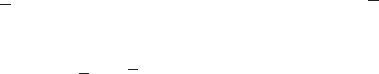
Figure 11.6 shows calculated distributions of horizontal velocity, u,

and longitudinal stress deviator, σ



,inthe reference model. A zone of

high u and σ



is present just below the water line near the calving face.

We hypothesized that this would tend to produce an overhang in the face,

and that this might facilitate calving. As a measure of the rate of overhang

development, we calculated the velocity gradient, du/dz, between this

point of maximum velocity and the bed (where the glacier was sliding).

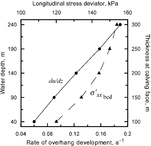
Comparison of models with total calving-face heights ranging from 100

to 300 m, all of which had subaerial heights of 60 m, suggested that,

in nature, du/dz probably increases nearly linearly with water depth

(Figure 11.7). In addition, the rate of stretching along the bed just

upglacier from the calving face, σ



bed

, increases with water depth

(Figure 11.7). The latter may facilitate the formation of bottom crevasses,

and hence submarine calving. The two effects, combined, provide a plau-

sible physical explanation for the empirical relation, Equation (11.14).

Role of permafrost in ice sheet dynamics and

landform evolution

For decades, glacial geologists have speculated on the effects that bed

conditions have on ice sheet proﬁles and dynamics (see, for example,

Matthews, 1974;Fisher et al., 1985) and on the relation between basal

306 Numerical modeling

Distance from calving face, m

1200

1210

1220

1230

1240

1250

1260

Height, mHeight, m

200

150

100

230

200

100

400500 300 200 100 0

200

150

100

(a)

(b)

Water

level

140 m

Water

level

140 m

Figure 11.6. Contours of

(a) horizontal velocity and

(b) σ ’

in a glacier 200 m

thick at the calving face,

calculated with the use of a

ﬁnite-element model.

(Reproduced from Hanson

and Hooke, 2000. Used with

permission of the authors and

the International Glaciological

Society.)

thermal conditions and glacial landforms (see, for example, Moran et al.,

1980; Mooers, 1990b; Attig et al., 1989). Models of increasing sophis-

tication have been used to study these effects. Here we discuss a recent

time-dependent modeling effort by Cutler et al.(2000), using a ﬂow-band

ﬁnite-element model.

The modeled domain was a ∼1700 km ﬂow band extending from

James Bay in Canada across the eastern end of Lake Superior and down

the axis of the Green Bay lobe in Wisconsin to a Late Glacial Maximum

terminal moraine and beyond. This ﬂow band was chosen because ice-

wedge casts and similar features demonstrate that permafrost was present

along the margin in Wisconsin, and the modeling team wanted to estimate

the thickness and horizontal extent, measured along a ﬂowline extending

upglacier from the margin, of the submarginal permafrost zone. Their

ultimate goal was to investigate the role that permafrost may have played

in the development of certain landforms.

The model domain was broken into ∼100 columns with 50 nodes in

the ice and 75 nodes in the substrate – a total of nearly 9000 nodes when

the ice sheet extended to the terminal moraine. The particular model

Examples 307

Figure 11.7. Variation of the

rate of overhang development

and of σ ’

at bed with water

depth. Subaerial part of

calving face was 60 m high in

all simulations. (Reproduced

from Hanson and Hooke,

2000. Used with permission of

the authors and the

International Glaciological

Society.)

run discussed here began at 55 ka, with ice already covering the ﬁrst

275 km of the ﬂowline, and ran to 21 ka, the Late Glacial Maximum.

Time steps were 25 years. The model was forced with a mass balance

pattern that depended on mean annual temperature and precipitation,

and on the daily temperature range. The latter was essential to ensure

melting when the mean daily temperature was still a few degrees below

◦

C. Temperature and precipitation were speciﬁed at the margin and

were assumed to decrease in speciﬁed ways with increasing elevation

and latitude along the ice sheet surface. The variation in margin tem-

perature with time was based on well-dated paleoclimate studies (Figure

11.8a). Included in the model is a routine for keeping track of the amount

of meltwater produced by subglacial melt and lost by ﬂow through sub-

glacial aquifers. The viscous energy dissipated by this groundwater ﬂow

was added to the geothermal ﬂux. Divergence of the ice ﬂow was not

included.

Results of the model run are shown in Figure 11.8b−e.Figure 11.8b

shows proﬁles of the ice sheet at eight times between 48 and 21 ka,

and Figure 11.8c shows the ice extent as a function of time. The abrupt

decrease in thickness of the ice sheet at distances greater than about

900 km from the divide (Figure 11.8b)isaconsequence of the transition

in the bed from crystalline rocks to a deformable substrate at ∼30 ka

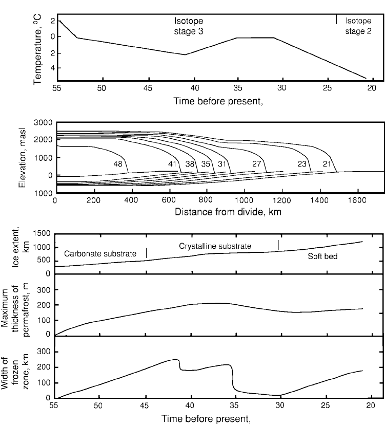
308 Numerical modeling

(a)

(b)

(c)

(d)

(e)

−

Figure 11.8. Model of a ﬂowline down the axis of the Green Bay lobe of the

Laurentide Ice Sheet. (a) Temperature speciﬁed at the margin from 55 to 20 ka.

(b) Proﬁles of the ice sheet at eight times between 48 and 21 ka (numbers to left

of curves). (c) Location of margin as a function of time. (d) Maximum thickness

of permafrost. (e) Width of submarginal frozen zone measured upglacier from

margin along the ﬂowline. (Redrawn from Cutler et al., 2000, Figures 3, 9, and

11. Used with permission of the authors and the International Glaciological

Society.)

Examples 309

(Figure 11.8c). Basal sliding was allowed only over the latter and only

when the bed was at the pressure melting point. With sliding, the balance

velocity (Equation (5.1)) is reached with thinner ice and a lower driving

stress (ρghα). Note the progressive isostatic depression of the bed as

the ice advances (Figure 11.8b) and the acceleration of the advance over

the soft deformable bed (Figure 11.8c). Figures 11.8d and 11.8e show the

maximum thickness of the permafrost and the width (measured along

the ﬂowline) of the submarginal frozen zone (see Figure 6.16). The

permafrost is thickest when the glacier margin ﬁrst reaches a given place

on the landscape, and then thins as the ice cover thickens and insulates

the site from the climate. The initial increase in maximum thickness is a

response to the cooling climate (Figure 11.8a). The subsequent decrease

from about 35 to 30 ka (Figure 11.8d)isadelayed reaction to the cli-

matic amelioration that began at 40 ka. The width of the subglacial frozen

zone reﬂects a balance between the rate of increase in width as the ice

sheet advances over permafrost and the rate of decrease in width as the

upglacier edge of the permafrost thaws. Changes in width thus result from

a combination of changes in rate of advance and changes in climate: the

decrease in rate of advance at ∼38 ka (Figure 11.8c) results in a decrease

in width (Figure 11.8e), and the increase in rate of advance at ∼30 ka

results in an increase in width. The abrupt ∼70 km decrease in width

at ∼42 ka is puzzling, but both it and the abruptness of the decrease at

35 ka suggest that at the upglacier edge there was a wide zone of relatively

thin permafrost that disappeared nearly simultaneously.

Cutler et al. (2000) reach three basic conclusions from this study.

Permafrost persists for time spans of order 10

–10

years beneath an

advancing ice margin.

The maximum width of the submarginal permafrost zone is of order

km.

Submarginal permafrost severely inhibits drainage of basal meltwater,

leading to high subglacial water pressures.

Although the dimensions of the permafrost layer (as well as many other

model results) are sensitive to the values of the parameters used to deﬁne

the climate, substrate characteristics, and sliding speed, these results

appear to be robust; the modeled Late Glacial Maximum (LGM) ice sheet

had a wide, persistent frozen toe with all tested values of the parameters.

Acaveat is that in their sensitivity studies Cutler et al.varied only one

input parameter at a time. Their conclusion would be stronger if they had

varied two or more parameters simultaneously in a direction to minimize

the width of the frozen zone.

The probable existence of such a frozen margin during the LGM has

several geomorphic implications.

310 Numerical modeling

As the width of the frozen margin decreases, rather abrupt releases of

stored subglacial water are likely. This supports the authors’ hypothesis

that tunnel valleys found along the LGM margin in Wisconsin were

formed by such drainage.

High subglacial water pressures are likely, so landforms associated

with deforming beds are to be expected. Bands of drumlins upglacier

from the presumed zone of frozen bed in Wisconsin (Attig et al., 1989)

are consistent with this, inasmuch as a mobile substrate appears to be

an essential requirement for drumlin formation (Patterson and Hooke,

1995).

Thrust features formed by the mechanism discussed in Chapter 6

(Figure 6.16) might be expected but somewhat surprisingly are not

found in Wisconsin. Such features are present at comparable latitudes

in neighboring states.

Large proglacial lakes like those that formed between the advancing ice

margin and the southern shores of Lakes Michigan and Erie would have

inhibited formation of submarginal permafrost. This may explain, in

part, why features such as drumlins, thrust features, and tunnel valleys

are rare or absent south of these lakes, but higher marginal temperatures

would also be a factor. It may also explain why ice lobes that ﬁlled

these lakes extended further south.

While glacial geologists had speculated that permafrost might persist

for some time under the margins of advancing continental ice sheets

(see, for example, Mickelson, 1987), numerical modeling such as that

carried out by Cutler et al. provides a much ﬁrmer theoretical basis for

this speculation.

Three-dimensional models of ice sheets

Recently, glaciologists have put considerable effort into modeling entire

ice sheets like those in Greenland and Antarctica. The results of some

of these models have already been presented in Figures 5.2, 6.14, and

6.15.Armed with models that closely reproduce the characteristics of

these modern ice sheets, one can examine the conditions under which

past ice sheets expanded to lower latitudes, or predict the behavior of

present ice sheets under various scenarios for climate change in the

future.

An interesting application of a three-dimensional thermomechanical

ﬁnite-difference model of a continental ice sheet is that of Marshall et al.

(2000), who studied the Laurentide Ice Sheet. The model run starts

at 122 ka, and is forced by a paleoclimate scenario based on a global