Hooke R.L. Principles of glacier mechanics

Подождите немного. Документ загружается.

Solutions for stresses and velocities 281

not necessarily valid at the ends of the slab. Note also that between

any two vertical sections, x

and x

+ x, u increases by b

x/h,which

would be the increase in mean velocity required to transmit the additional

ﬂux, b

x,downglacier – the balance velocity that we discussed in

Chapter 5.

If there is no accumulation or ablation, b

= 0, and thus u = c and

w = 0 throughout the block. In this case there is no internal deformation.

All movement is conﬁned to sliding. The yield criterion is then satisﬁed

only at the bed and σ

can take any value between the limits shown in

Figure 10.2.

Stress and velocity solutions for a nonlinear material

Let us now relax the assumption that the material with which we are

dealing is perfectly plastic, and instead allow it to have a nonlinear rhe-

ology, as is the case with real ice. We will still consider a slab of inﬁnite

extent and uniform thickness resting on a bed with a uniform slope.

The stress equations are not changed, so the solutions for the stresses

(Equations (10.18)) remain basically the same. However, now σ does

not have a limiting value, k, the yield stress, so some changes must be

made.

As before (Equations (10.18)), we note that σ

≈ σ

on the bed, as

both are dominated by the hydrostatic pressure. As σ  0atthebed,

it is clear from Equation (10.8) that σ ≈ σ

 (σ

− σ

) ≈ 0 there.

Again, this emphasizes that deformation at the bed is largely by simple

shear. Thus σ

→ σ on the bed, so we replace k with σ in Equations

(10.18). In other words, while we still require that σ and σ

be uniform

(independent of x)onthe bed, we do not require that they are necessarily

equal to some speciﬁc value, as in a yield stress. In general, of course, σ

is likely to increase with the budget gradient (Figure 3.7), as ﬂow rates

must then be higher. In addition, we make use of the fact that k/h = ρg

from the discussion following Equation (10.17). With these changes, the

stress solutions become:

=−ρg

z ± 2



− (ρg

=−ρg

z (10.30)

=−ρg

As before, the upper sign is for extending, and the lower for compressive

ﬂow.

In order to evaluate σ

(z), we need to know how σ varies with depth,

z. This will emerge in the course of obtaining the velocity solutions.

282 Stress and velocity distribution

To solve for the velocities, we start by combining the stress solutions

with Equations (10.5) through (10.7)toobtain:

∂u

∂x

=−

∂w

∂z

(

− σ

)

=±λ



− (ρg



∂u

∂z

∂w

∂x



= λσ

=−λρ g

(10.31)

As before (discussion preceding Equation (10.22)), because w = 0

on the lower boundary, and because w must thus be independent of

x everywhere to avoid discontinuities, ∂w/∂x = 0everywhere. Thus,

using the arguments outlined in Equations (10.22)–(10.24)weobtain, as

before:

w = c

z + c

(10.32)

The boundary conditions now are not as clear as they were earlier because

the thickness may change with time. Thus w = b

on z = 0.

From Equations (10.31) and (10.32)wehave:

∂w

∂z

= c

=−

∂u

∂x

(10.33)

Therefore, from the ﬁrst of Equations (10.31):

=∓λ



− (ρg

(10.34)

Using this to eliminate λ in the second of Equations (10.31) yields:

∂u

∂z

=±2ρg



− (ρg

(10.35)

As λ is deﬁned by ˙ε

= λσ



,itmust be positive if positive stresses are

to produce positive strain rates. To ensure that this is the case, we give

the values ∓r where r is a positive constant. From Equation (10.33)

it is clear that r is the longitudinal strain rate. Equation (10.33) thus

becomes:

∂u

∂x

=±r

The solution for w now becomes:

w =∓rz + c

Applying the boundary condition w = 0onz = h,weget c

=±rh, so:

w =∓r(z − h) =±rh



1 −



(10.36)

Note that w still varies linearly with depth as in the perfectly plas-

tic case, despite the variation in σ with depth. This is implicit in the

fact that the longitudinal strain rate is independent of depth, which in

turn results from the fact that stresses must be independent of x in a

Solutions for stresses and velocities 283

slab on a uniform slope (see discussion following Equation (10.21);

∂u/∂x =−∂w/∂z and by Equation (10.24), ∂w/∂z = constant).

To obtain u, integrate Equation (10.35) (with Equation (10.34)),

thus:

u =−2g



λρ zdz + f (x) (10.37)

Setting the derivative of this with respect to x equal to ±r, and integrating

gives f (x) =±rx +c. Combining this with Equation (10.37) and using

the boundary condition u = u

at x = z = 0 yields:

u =±rx − 2g



λρ zdz + u

(10.38)

The velocity, u

,atthe surface (z =0), is ±rx +u

. Here u

is the velocity

at the origin, x =0, and rx is the increase (or decrease) in velocity between

the origin and the point in question as a result of longitudinal straining.

In a real glacier, r = r(x), so one would have to integrate over x to obtain

in this way. In practice, we would be more likely to simply take u

as known. Accordingly, we will replace ±rx + u

with u

in Equation

(10.38).

To proceed further, we must assume a ﬂow law; as before, we use

˙ε = λσ = (σ/B)

with B and n constant, independent of position.

Hence,

λ =

n−1

(10.39)

and Equation (10.38) becomes (assuming that ρ is independent of depth):

u = u

−

2ρg



n−1

zdz (10.40)

To integrate this, σ must be expressed in terms of z.From Equation

(10.34) with c

=∓r:

λ =



− (ρg

n−1

Rearranging, this becomes:

z =

√

−r

ρg

n−1

(10.41)

whence:

dσ

nσ

2n−1

ρg

n−1

√

−r

− (n − 1)

√

−r

ρg

2(n−1)

n−2

nσ

ρg

√

−r

− (n − 1)

√

−r

ρg

284 Stress and velocity distribution

When z = 0, σ

= r

,orσ = r

1/n

B,soEquation (10.40)istobe

integrated from r

1/n

B to σ . Equation (10.40) thus becomes:

u = u

−

2ρg



1/n

√

−r

ρg



nσ

ρg

√

−r

− (n − 1)

√

−r

ρg



dσ

= u

−

ρg



1/n

[nσ

− (n − 1)σ

+ (n − 1)r

−n

]dσ

Carrying out the integration yields:

u = u

−

ρg

(n + 1)







− (n + 1)r

1−n

+ nr



(10.42)

which, together with Equation (10.41), provides the desired solution for

u in terms of z. Expressing u explicitly in terms of z is awkward. Rather,

it is better to assume a value of σ , and to use it to calculate the depth z

to that σ and the velocity at that depth.

When r = 0, these equations reduce to:

u = u

−

ρg

(n + 1)









and

z =

ρg

n−1

ρg

Thus:

u = u

−

n + 1



ρg



n+1

which is the same as Equation (5.6). A fundamental assumption made

in the derivation of Equation (5.6) should now be more meaningful:

namely that all strain rates other than shear strain parallel to the bed, ˙ε

were negligible. In deriving Equation (10.42)weadded only one addi-

tional strain rate, ˙ε

(= r), yet the complexity of the solution increased

signiﬁcantly.

Now that we have an expression relating σ and z,wecan plot stress

distributions from Equations (10.30). This is done in Figure 10.5 for a

glacier with a longitudinal strain rate of 0.1 a

−1

resting on a bed with a

slope of 0.1. As in the perfectly plastic case (Figure 10.2), σ

and σ

vary linearly with depth, while σ

varies nonlinearly and is also double

valued. Furthermore, for any given depth σ is a function of n (Equa-

tion (10.41)). Thus, σ

varies with n.Asn becomes large, the solution

for σ

converges on the elliptic distribution obtained earlier (Figure

10.2). For n = 1, σ (Equation (10.41)) and hence σ

(ﬁrst of Equa-

tions (10.30)) decrease linearly with depth. As P(=

(σ

+ σ

)) also

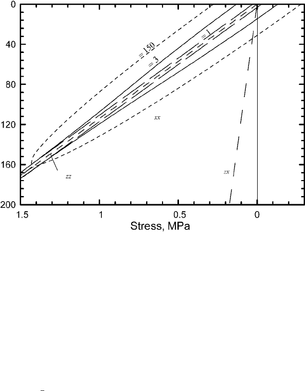
Solutions for stresses and velocities 285

Depth, m

Figure 10.5. Depth variation of stress in an ice sheet with a power law

rheology. The ice sheet consists of a slab of uniform thickness and density resting

on a bed with a slope of 0.1. The distribution of σ

is given by the pairs of curves

labeled with values of n. The distributions of σ

and σ

are the same for all n.

Calculations use n = 3, B = 0.141 MPa a

− 1/n

and r = 0.1 a

−1

.Asn →∞, the

thickness of the ice sheet is limited to h = B/ρg

, which in this case is ∼160 m.

decreases linearly with depth with the same constant of proportionality,

ρg

, σ



becomes independent of depth.

Further insight may be gained by considering the case when σ = 0.

If r = 0, z becomes indeﬁnite. This is because although σ

= 0atthe

surface, σ =

> 0 there. Thus, when there is longitudinal strain,

there is no place in the slab where σ = 0.

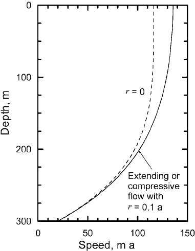
Twovelocity proﬁles calculated from Equations (10.41) and (10.42)

are shown in Figure 10.6. One proﬁle is calculated with r = 0, and

the other with r = 0.1 a

−1

. Note that u

is adjusted to yield u

= 20

−1

in both cases. One might initially think that the higher speed

represented by the dashed proﬁle in Figure 10.6 wasaconsequence of

longitudinal stretching. However, r is a positive constant (so a negative

value of r cannot be entered in Equation (10.42)) and ∂u/∂x =±r. Thus,

the dashed proﬁle is applicable to compressive ﬂow as well as extending

ﬂow. This is because the magnitude of the increase in σ , and hence in

λ, resulting from the addition of a longitudinal stress, is independent

of whether the longitudinal stress is compressive or extending. As λ

increases so does ˙ε

for any given σ

(Equation (9.29)). Speciﬁcally, ˙ε

(= ∂u/∂z) increases, regardless of whether σ

is positive or negative.

286 Stress and velocity distribution

−1

Figure 10.6. Velocity

proﬁles, calculated from

Equations (10.41) and

(10.42), in a glacier consisting

of an inﬁnite slab of ice,

300 m thick, resting on a bed

with a slope of 0.046 and

sliding with a speed, u

,of

20ma

−1

. Calculations use

n = 3 and B = 0.141 MPa a

−1/3

and two different values of r

as shown.

Comparison with real glaciers

Real glaciers are not slabs of ice of uniform thickness, nor are they

perfectly plastic. Thus, it is relevant to consider what aspects of the

solutions we have obtained are applicable in reality.

Consider ﬁrst the result that σ

and σ

vary linearly with depth.

Such a linear variation is often assumed in studies of real glaciers and is

a reasonable approximation in many situations.

In addition we found that, in general, ﬂow is extending in accumu-

lation areas and compressive in ablation areas. This is because r varies

directly with b

(if the glacier is not too far from a steady state), and σ

varies directly with r for any given depth (Equation (10.41)). Thus, σ

varies directly with b

, being positive when b

is positive and conversely.

In an actual glacier, however, longitudinal stresses also depend on factors

such as the curvature of the longitudinal surface proﬁle and the rate of

change in thickness. Thus, it is not productive to try to calculate longitu-

dinal stresses in a real glacier with the use of the theory presented here.

The physical processes by which the longitudinal strain rate is

adjusted to balance b

can be visualized qualitatively. If, in some loca-

tion, r is too large so that thinning by extension exceeds thickening by

accumulation, the proﬁle will tend to become concave and this will have

a tendency to decrease r.

Summary 287

Also relevant to real glaciers is the effect of longitudinal stress on

velocities. Clearly, longitudinal compression should result in upward

vertical velocities, and conversely. The linear decrease in w with depth,

however, is an artifact of our slab model (see discussion following Equa-

tion (10.36)), although it is an approximation that is commonly used in

calculations, as we noted in Chapter 5.With respect to vertical proﬁles

of u, longitudinal stresses, whether extending or compressive, increase

the effective stress, so they increase ∂u/∂z throughout the proﬁle. This

may be particularly evident near a glacier surface where σ

is small so

˙ε

would be negligible were it not for the contribution of σ

to σ .We

will ﬁnd in Chapter 12,however, that certain peculiarities of measured

deformation proﬁles cannot be explained in this way.

Summary

In this chapter, we have shown that Equations (9.32) can be solved for

the three components of the velocity vector and nine components of the

stress tensor in certain simple situations. Our solutions were for a slab

of inﬁnite horizontal extent resting on a bed with a uniform slope. We

ﬁrst obtained a solution for a perfectly plastic material, and found that

the thickness of the slab was constrained by the yield strength of the

material. We then obtained solutions for a nonlinear material which are

more relevant to real glaciers.

We found that σ

and σ

vary linearly with depth, which is probably a

reasonable approximation to the situation in many real glaciers. We also

found that longitudinal stresses should be extending in accumulation

areas and compressive in ablation areas, although the magnitude of the

longitudinal stresses is not well constrained by our simple model.

Ver tical velocities vary linearly with depth for the idealized situation

that we studied, and this is commonly used as a ﬁrst approximation in

real glaciers (e.g. Equation 6.15). Horizontal velocities decrease nonlin-

early with depth, as we found in Chapter 5.Inthis chapter, however, we

were able to investigate the effect of longitudinal stresses on the veloc-

ity proﬁle, and found that either longitudinal extension or longitudinal

compression will increase ∂u/∂z, leading to higher velocities.

Chapter 11

Numerical modeling

On several occasions when we encountered problems that could not be

solved readily by analytical methods, we have referred to results from

numerical models. In Chapters 5 and 10 we found, in fact, that analytical

solutions to problems of glacier ﬂow could be obtained only when the

problems were quite simple. The two numerical methods that are most

commonly used in modeling are the ﬁnite-difference and ﬁnite-element

methods.

The analytical methods of calculus are based on taking the limit as

intervals over which functions are evaluated are allowed to shrink toward

zero. In ﬁnite-difference and ﬁnite-element models, in contrast, we let

these intervals remain ﬁnite and assume that the functions describing

the variation of parameters across them can be replaced by constants, by

linear functions, or by low-order polynomials. The resulting equations

turn out to be much simpler than the original differential equations, but

because the domain of interest is now broken into many small inter-

vals, one must do a large number of repetitive calculations to obtain a

solution for the entire domain. Computers are thus used for all but the

simplest numerical calculations. Moreover, the numerical solutions are

not necessarily as accurate as analytical ones.

In this chapter, we ﬁrst describe elementary numerical integration.

This leads into some straightforward ﬁnite-difference calculations that

can be carried out with the use of a spread sheet, a short computer

program, or available mathematical software. The numerical details of

more advanced ﬁnite-difference models and of ﬁnite-element models

are beyond the scope of this book. However, we will discuss some of the

288

Numerical integration 289

techniques used in these models, and then illustrate the use of models

with a few examples.

Goals of modeling

“Solving” a mathematical problem analytically usually means ﬁnding

values for one or more unknown quantities. This is true, also, of solutions

using numerical models. In typical problems with several unknowns, for

example, numerical models are commonly used to explore the universe

of physically reasonable values of the unknowns, and thus determine

which combinations give satisfactory agreement with observations. An

example is a study of a temperature proﬁle measured in a borehole that

penetrated the Greenland Ice Sheet at Dye 3, where the ice is 2037 m thick

(Dahl-Jensen and Johnsen, 1986). The three unknowns, or free variables,

were the Pleistocene accumulation rate, Pleistocene surface temperature,

and geothermal heat ﬂux. It was found that these could be constrained to

lie, respectively, between 33% and 75% of the present accumulation rate,

−30 and −35

◦

C (12

◦

C below the present mean annual temperature),

and 31 and 45 mW m

−2

.Ifthe model took all signiﬁcant processes into

consideration and did so accurately, these values are “solutions” for the

three unknowns. More precise solutions are not possible because equally

good matches to the observed temperature proﬁle can be obtained with

several combinations of these three parameters within the above limits.

The observations that one seeks to match need not necessarily be

quantitative measurements. An exciting approach that is being used with

increasing frequency and sophistication is the use of observations of the

distribution of glacial landforms to constrain models of vanished ice

sheets and, in turn, to support hypotheses regarding the origin of the

landforms. Moraines obviously provide information on the extent of an

ice sheet, and some glacial landforms, as we have discussed, appear to

require a certain basal thermal regime. Combinations of model param-

eters that yield ice sheets of this size and with this basal temperature

distribution are thus more likely to represent reality.

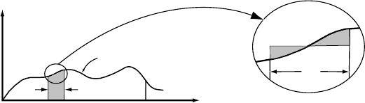
Numerical integration

Consider a differential equation of the form:

dϕ

= f (x)

with the solution:

ϕ =



f (x) dx (11.1)

290 Numerical modeling

(x)

f (x)

∆x

(a)

∆x

(b)

Figure 11.1. (a) Illustration

of a numerical integration to

obtain the area under a curve.

(b) Detail of the circled area in

(a). See text for discussion.

If f (x)isthe curve shown in Figure 11.1a, for example, ϕ is the area

under the curve between 0 and X.Ifthe function f (x) can be integrated

analytically, ϕ is easily obtained. However, if f (x) cannot be integrated

analytically we can still carry out the integration numerically. (Numerical

integration is sometimes called quadrature.) To do this, ﬁrst divide the

interval 0 → X into n segments of equal length, x, and then evaluate

the sum:

ϕ =



i=1

f (x

)x (11.2)

This sum can be obtained by evaluating f (x)atthe midpoint of every

interval x, multiplying by x, and adding the results. The shaded area

in Figure 11.1a would be one such product f (x)x. This procedure makes

use of the fact that an integral is the limit as x → 0ofthe summation

in Equation (11.2).

A common alternative to this is to evaluate f (x)atthe beginning and

end of every interval, x, and then multiply x by the average of these

two values. Because this approximates the shaded area as a trapezoid, it

is called trapezoidal integration.

Neither solution for ϕ is exact. To see why this is the case, consider

Figure 11.1b,which is an enlargement of the circled area in Figure 11.1a.

The point labeled “A”isf (x)atthe midpoint of the interval x. The

product f (x)x overestimates the area under the curve in the interval x

by the size of the shaded area to the left of A and underestimates it by

the size of the shaded area to the right of A.Inthis particular instance,

the latter is larger, so the area under the curve is underestimated. The

magnitude of the ﬁnal error will depend upon the sum of these individual

errors. The smaller the intervals x, the closer the numerical solution

will be to the exact solution.

More sophisticated techniques for numerical integration are also

available. For example, the shape of a curve between two points may

be approximated by a polynomial (Irons and Shrive, 1987, pp. 64–67).

This technique, sometimes called Gaussian quadrature, produces highly