Hjorth-Jensen M. Computational Physics

Подождите немного. Документ загружается.

13.4. PHYSICS PROJECTS: BOUND STATES IN MOMENTUM SPACE 249

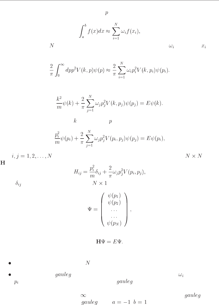
First we need to evaluate the integral over using e.g., gaussian quadrature. This means that

we rewrite an integral like

where we have ﬁxed lattice points through the corresponding weights and points . The

integral in Eq. (13.48) is rewritten as

(13.49)

We can then rewrite the SE as

(13.50)

Using the same mesh points for

as we did for in the integral evaluation, we get

(13.51)

with

. This is a matrix eigenvalue equation and if we deﬁne an matrix

to be

(13.52)

where

is the Kronecker delta, and an vector

(13.53)

we have the eigenvalue problem

(13.54)

The algorithm for solving the last equation may take the following form

Fix the number of mesh points .

Use the function in the program library to set up the weights and the points

. Before you go on you need to recall that uses the Legendre polynomials to ﬁx

the mesh points and weights. This means that the integral is for the interval [-1,1]. Your

integral is for the interval [0,

]. You will need to map the weights from to your

interval. To do this, call ﬁrst , with , . It returns the mesh points and

250 CHAPTER 13. EIGENSYSTEMS

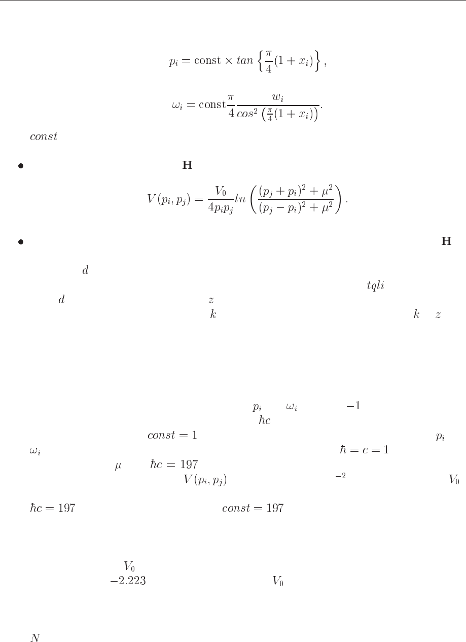
weights. You then map these points over to the limits in your integral. You can then use

the following mapping

and

is a constant which we discuss below.

Construct thereafter the matrix with

We are now ready to obtain the eigenvalues. We need ﬁrst to rewrite the matrix in

tri-diagonal form. Do this by calling the library function tred2. This function returns

the vector

with the diagonal matrix elements of the tri-diagonal matrix while e are the

non-diagonal ones. To obtain the eigenvalues we call the function

. On return, the

array contains the eigenvalues. If is given as the unity matrix on input, it returns the

eigenvectors. For a given eigenvalue , the eigenvector is given by the column in , that

is z[][k] in C, or z(:,k) in Fortran 90.

The problem to solve

1. Before you write the main program for the above algorithm make a dimensional analysis

of Eq. (13.48)! You can choose units so that

and are in fm . This is the standard

unit for the wave vector. Recall then to insert in the appropriate places. For this case

you can set the value of

. You could also choose units so that the units of and

are in MeV. (we have previously used so-called natural units ). You will then

need to multiply with MeVfm to obtain the same units in the expression for

the potential. Why? Show that

must have units MeV . What is the unit of ?

If you choose these units you should also multiply the mesh points and the weights with

. That means, set the constant .

2. Write your own program so that you can solve the SE in momentum space.

3. Adjust the value of

so that you get close to the experimental value of the binding energy

of the deuteron,

MeV. Which sign should have?

4. Try increasing the number of mesh points in steps of 8, for example 16, 24, etc and see

how the energy changes. Your program returns equally many eigenvalues as mesh points

. Only the true ground state will be at negative energy.

13.5. PHYSICS PROJECTS: QUANTUM MECHANICAL SCATTERING 251

13.5 Physics projects: Quantum mechanical scattering

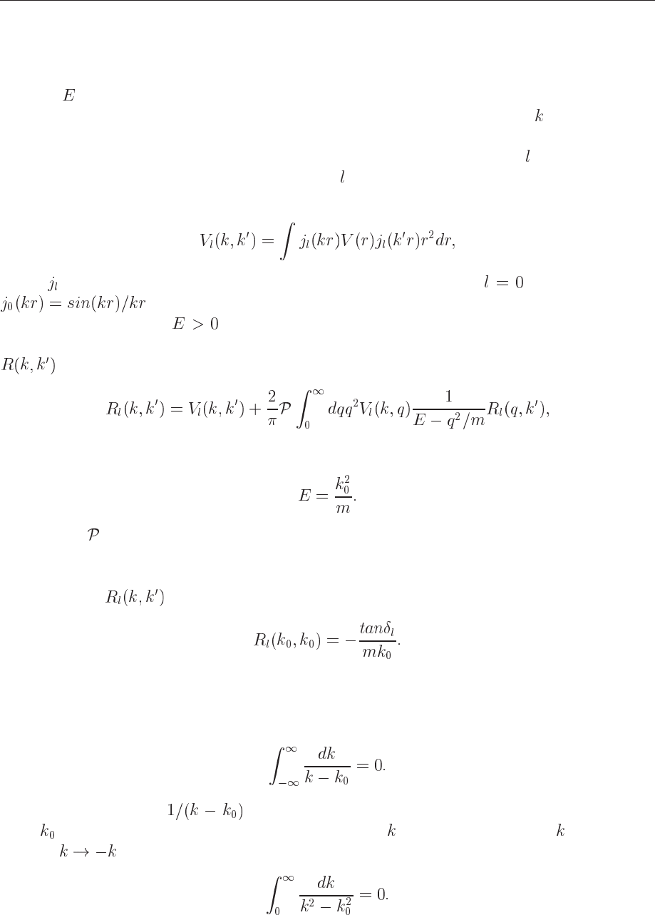
We are now going to solve the SE for the neutron-proton system in momentum space for positive

energies

in order to obtain the phase shifts. In the previous physics project on bound states

in momentum space, we obtained the SE in momentum space by Eq. (13.48).

was the relative

momentum between the two particles. A partial wave expansion was used in order to reduce the

problem to an integral over the magnitude of momentum only. The subscript referred therefore

to a partial wave with a given orbital momentum

. To obtain the potential in momentum space

we used the Fourier-Bessel transform (Hankel transform)

(13.55)

where

is the spherical Bessel function. We will just study the case , which means that

For scattering states,

, the corresponding equation to solve is the so-called Lippman-

Schwinger equation. This is an integral equation where we have to deal with the amplitude

(reaction matrix) deﬁned through the integral equation

(13.56)

where the total kinetic energy of the two incoming particles in the center-of-mass system is

(13.57)

The symbol

indicates that Cauchy’s principal-value prescription is used in order to avoid the

singularity arising from the zero of the denominator. We will discuss below how to solve this

problem. Eq. (13.56) represents then the problem you will have to solve numerically.

The matrix

relates to the the phase shifts through its diagonal elements as

(13.58)

The principal value in Eq. (13.56) is rather tricky to evaluate numerically, mainly since com-

puters have limited precision. We will here use a subtraction trick often used when dealing with

singular integrals in numerical calculations. We introduce ﬁrst the calculus relation

(13.59)

It means that the curve

has equal and opposite areas on both sides of the singular

point . If we break the integral into one over positive and one over negative , a change of

variable

allows us to rewrite the last equation as

(13.60)

252 CHAPTER 13. EIGENSYSTEMS

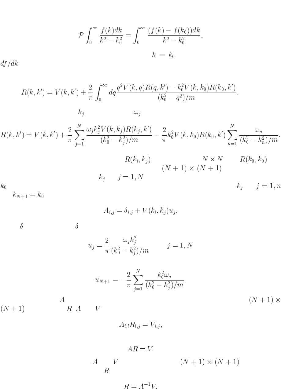
We can use this to express a principal values integral as

(13.61)

where the right-hand side is no longer singular at

, it is proportional to the derivative

, and can be evaluated numerically as any other integral.

We can then use the trick in Eq. (13.61) to rewrite Eq. (13.56) as

(13.62)

Using the mesh points

and the weights , we can rewrite Eq. (13.62) as

(13.63)

This equation contains now the unknowns (with dimension ) and . We

can turn Eq. (13.63) into an equation with dimension

with a mesh which

contains the original mesh points for and the point which corresponds to the energy

. Consider the latter as the ’observable’ point. The mesh points become then for

and . With these new mesh points we deﬁne the matrix

(13.64)

where

is the Kronecker and

(13.65)

and

(13.66)

With the matrix

we can rewrite Eq. (13.63) as a matrix problem of dimension

. All matrices , and have this dimension and we get

(13.67)

or just

(13.68)

Since we already have deﬁned

and (these are stored as matrices) Eq.

(13.68) involves only the unknown . We obtain it by matrix inversion, i.e.,

(13.69)

13.5. PHYSICS PROJECTS: QUANTUM MECHANICAL SCATTERING 253

Thus, to obtain , we need to set up the matrices and and invert the matrix . To do that one

can use the function matinv in the program library. With the inverse

, performing a matrix

multiplication with results in .

With we obtain subsequently the phaseshifts using the relation

(13.70)

Chapter 14

Differential equations

14.1 Introduction

Historically, differential equations have originated in chemistry, physics and engineering. More

recently they have also been used widely in medicine, biology etc. In this chapter we restrict

the attention to ordinary differential equations. We focus on initial value and boundary value

problems and present some of the more commonly used methods for solving such problems

numerically.

The physical systems which are discussed range from a simple cooling problem to the physics

of a neutron star.

14.2 Ordinary differential equations (ODE)

In this section we will mainly deal with ordinary differential equations and numerical methods

suitable for dealing with them. However, before we proceed, a brief remainder on differential

equations may be appropriate.

The order of the ODE refers to the order of the derivative on the left-hand side in the

equation

(14.1)

This equation is of ﬁrst order and is an arbitrary function. A second-order equation goes

typically like

(14.2)

A well-known second-order equation is Newton’s second law

(14.3)

where

is the force constant. ODE depend only on one variable, whereas

255

256 CHAPTER 14. DIFFERENTIAL EQUATIONS

partial differential equations like the time-dependent Schrödinger equation

(14.4)

may depend on several variables. In certain cases, like the above equation, the wave func-

tion can be factorized in functions of the separate variables, so that the Schrödinger equa-

tion can be rewritten in terms of sets of ordinary differential equations.

We distinguish also between linear and non-linear differential equation where e.g.,

(14.5)

is an example of a linear equation, while

(14.6)

is a non-linear ODE. Another concept which dictates the numerical method chosen for

solving an ODE, is that of initial and boundary conditions. To give an example, in our

study of neutron stars below, we will need to solve two coupled ﬁrst-order differential

equations, one for the total mass

and one for the pressure as functions of

and

where is the mass-energy density. The initial conditions are dictated by the mass being

zero at the center of the star, i.e., when

, yielding . The other condition

is that the pressure vanishes at the surface of the star. This means that at the point where

we have in the solution of the integral equations, we have the total radius of

the star and the total mass

. These two conditions dictate the solution of the

equations. Since the differential equations are solved by stepping the radius from

to , so-called one-step methods (see the next section) or Runge-Kutta methods may

yield stable solutions.

In the solution of the Schrödinger equation for a particle in a potential, we may need to

apply boundary conditions as well, such as demanding continuity of the wave function and

its derivative.

In many cases it is possible to rewrite a second-order differential equation in terms of two

ﬁrst-order differential equations. Consider again the case of Newton’s second law in Eq.

(14.3). If we deﬁne the position

and the velocity as its

derivative

(14.7)

14.3. FINITE DIFFERENCE METHODS 257

we can rewrite Newton’s second law as two coupled ﬁrst-order differential equations

(14.8)

and

(14.9)

14.3 Finite difference methods

These methods fall under the general class of one-step methods. The algoritm is rather simple.

Suppose we have an initial value for the function

given by

(14.10)

We are interested in solving a differential equation in a region in space [a,b]. We deﬁne a step

by splitting the interval in sub intervals, so that we have

(14.11)

With this step and the derivative of

we can construct the next value of the function at

(14.12)

and so forth. If the function is rather well-behaved in the domain [a,b], we can use a ﬁxed step

size. If not, adaptive steps may be needed. Here we concentrate on ﬁxed-step methods only. Let

us try to generalize the above procedure by writing the step in terms of the previous step

(14.13)

where represents the truncation error. To determine , we Taylor expand our function

(14.14)

where we will associate the derivatives in the parenthesis with

(14.15)

We deﬁne

(14.16)

and if we truncate

at the ﬁrst derivative, we have

(14.17)

258 CHAPTER 14. DIFFERENTIAL EQUATIONS

which when complemented with forms the algorithm for the well-known Euler

method. Note that at every step we make an approximation error of the order of

, however

the total error is the sum over all steps , yielding thus a global error which goes like

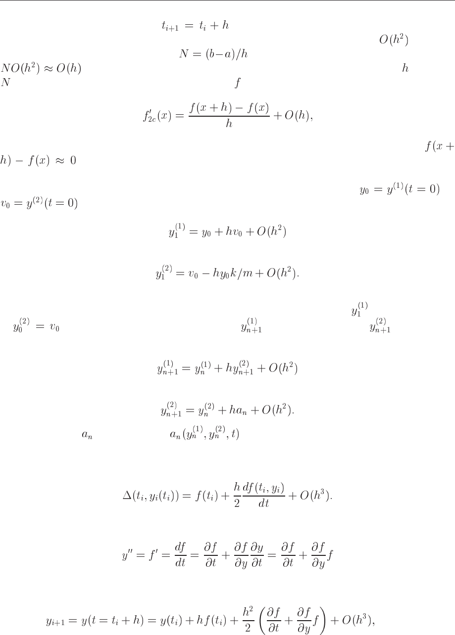
. To make Euler’s method more precise we can obviously decrease (increase

). However, if we are computing the derivative numerically by e.g., the two-steps formula

we can enter into roundoff error problems when we subtract two almost equal numbers

. Euler’s method is not recommended for precision calculation, although it is

handy to use in order to get a ﬁrst view on how a solution may look like. As an example,

consider Newton’s equation rewritten in Eqs. (14.8) and (14.9). We deﬁne

. The ﬁrst steps in Newton’s equations are then

(14.18)

and

(14.19)

The Euler method is asymmetric in time, since it uses information about the derivative at the

beginning of the time interval. This means that we evaluate the position at

using the velocity

. A simple variation is to determine using the velocity at , that is (in a

slightly more generalized form)

(14.20)

and

(14.21)

The acceleration

is a function of and needs to be evaluated as well. This is the

Euler-Cromer method.

Let us then include the second derivative in our Taylor expansion. We have then

(14.22)

The second derivative can be rewritten as

(14.23)

and we can rewrite Eq. (14.14) as

(14.24)