Hjorth-Jensen M. Computational Physics

Подождите немного. Документ загружается.

12.3. SIMULATION OF MOLECULAR SYSTEMS 229

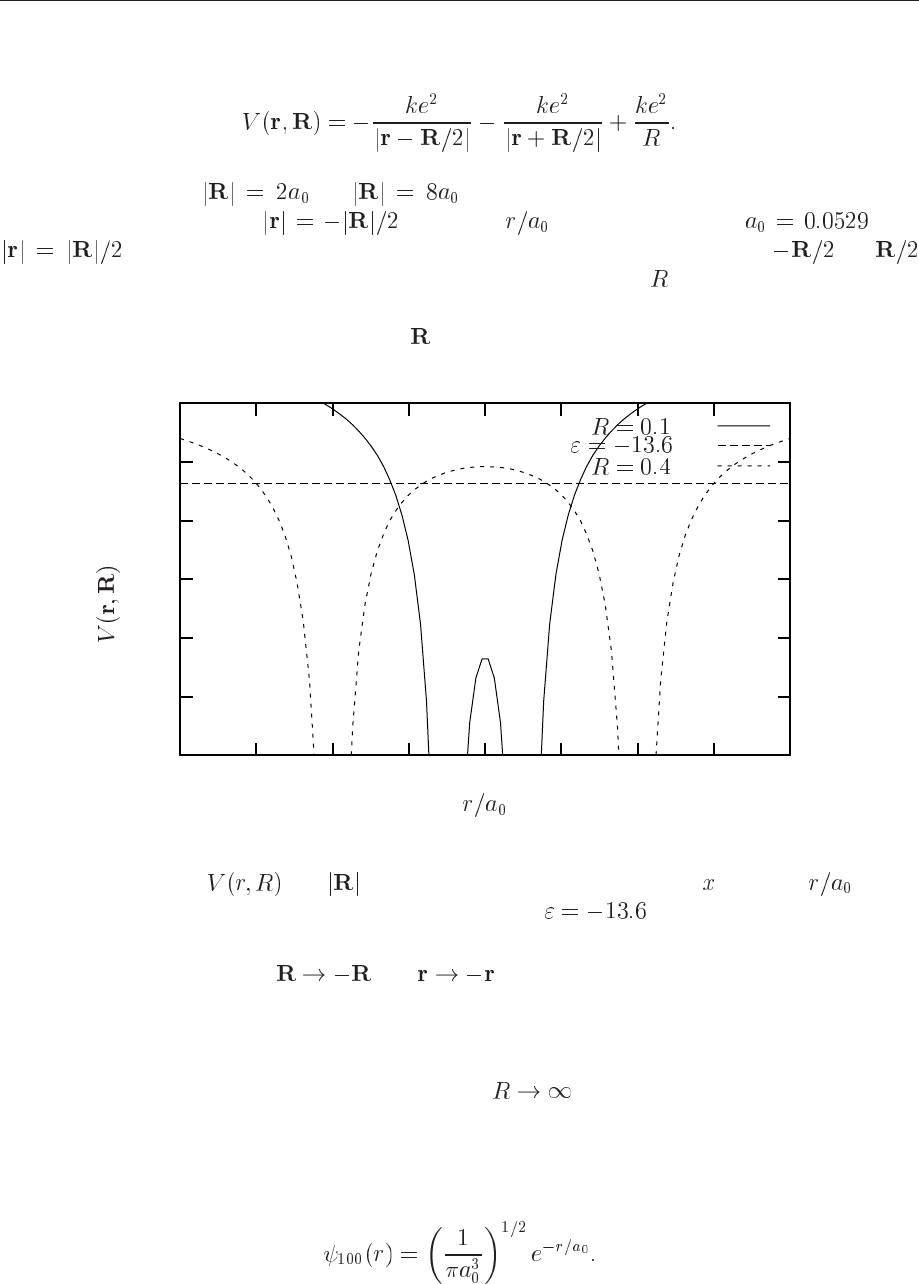
protons. In Fig. 12.5 we show a plot of the potential energy

(12.77)

Here we have ﬁxed

og , being 2 and 8 Bohr radii, respectively. Note

that in the region between (units are in this ﬁgure, with ) and

the electron can tunnel through the potential barrier. Recall that og

correspond to the positions of the two protons. We note also that if is increased, the potential

becomes less attractive. This has consequences for the binding energy of the molecule. The

binding energy decreases as the distance

increases. Since the potential is symmetric with

[eV]

-2-4

-6-8

-10

-20

-30

-40

-50

-60

Figure 12.5: Plot of

for =0.1 and 0.4 nm. Units along the -axis are . The

straight line is the binding energy of the hydrogen atom, eV.

respect to the interchange of

and it means that the probability for the electron

to move from one proton to the other must be equal in both directions. We can say that the

electron shares it’s time between both protons.

With this caveat, we can now construct a model for simulating this molecule. Since we have

only one elctron, we could assume that in the limit

, i.e., when the distance between the

two protons is large, the electron is essentially bound to only one of the protons. This should

correspond to a hydrogen atom. As a trial wave function, we could therefore use the electronic

wave function for the ground state of hydrogen, namely

(12.78)

230 CHAPTER 12. QUANTUM MONTE CARLO METHODS

Since we do not know exactly where the electron is, we have to allow for the possibility that

the electron can be coupled to one of the two protons. This form includes the ’cusp’-condition

discussed in the previous section. We deﬁne thence two hydrogen wave functions

(12.79)

and

(12.80)

Based on these two wave functions, which represent where the electron can be, we attempt at the

following linear combination

(12.81)

with

a constant.

12.3.2 Physics project: the H

molecule

in preparation

12.4 Many-body systems

12.4.1 Liquid

Liquid

He is an example of a so-called extended system, with an inﬁnite number of particles.

The density of the system varies from dilute to extremely dense. It is fairly obvious that we

cannot attempt a simulation with such degrees of freedom. There are however ways to circum-

vent this problem. The usual way of dealing with such systems, using concepts from statistical

Physics, consists in representing the system in a simulation cell with e.g., periodic boundary

conditions, as we did for the Ising model. If the cell has length

, the density of the system is

determined by putting a given number of particles

in a simulation cell with volume . The

density becomes then .

In general, when dealing with such systems of many interacting particles, the interaction it-

self is not known analytically. Rather, we will have to rely on parametrizations based on e.g.,

scattering experiments in order to determine a parametrization of the potential energy. The in-

teraction between atoms and/or molecules can be either repulsive or attractive, depending on the

distance

between two atoms or molecules. One can approximate this interaction as

(12.82)

where

are some integers and constans with dimension energy and length, and with

units in e.g., eVnm. The constants and the integers are determined by the constraints

12.4. MANY-BODY SYSTEMS 231

[nm]

0.50.450.40.350.30.25

0.007

0.006

0.005

0.004

0.003

0.002

0.001

-0.001

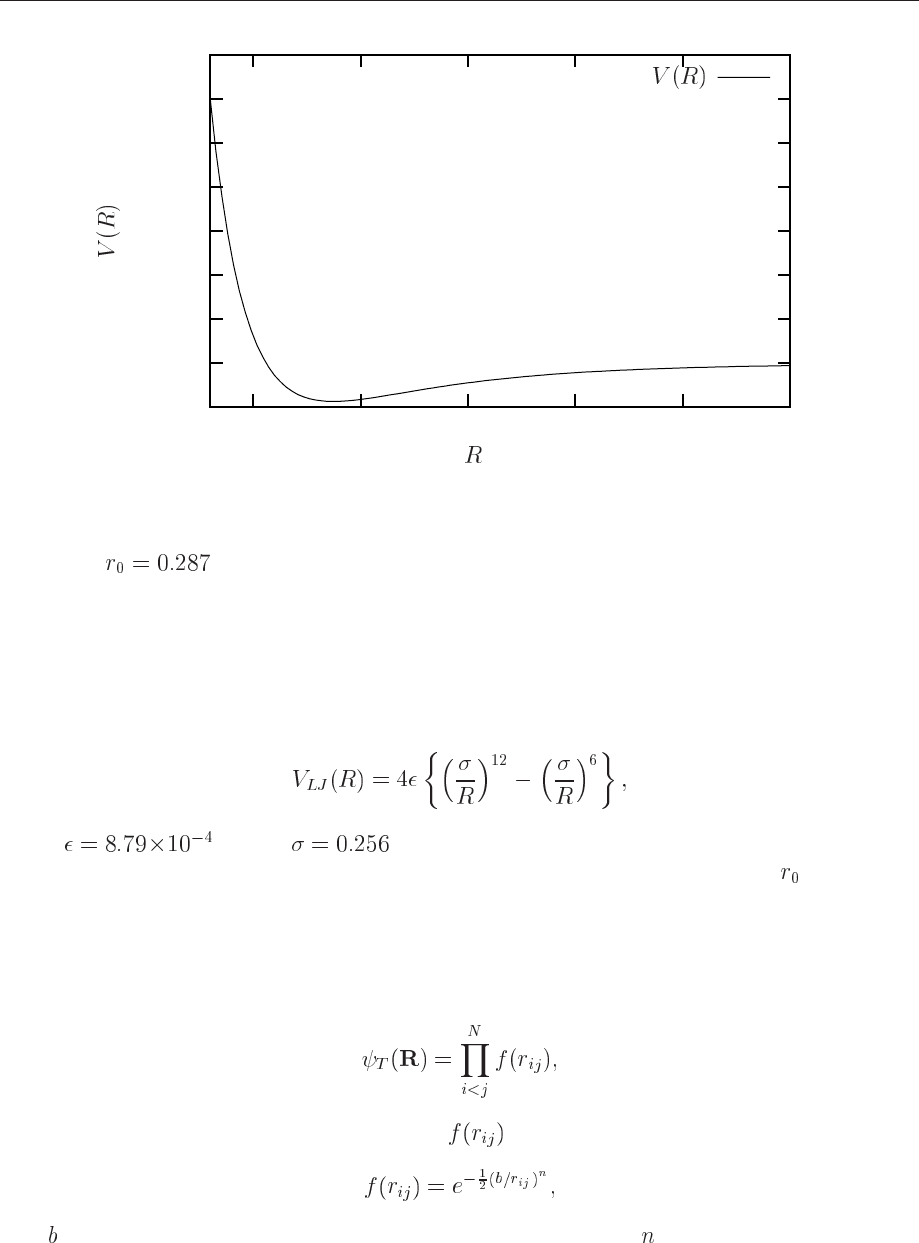
Figure 12.6: Plot for the Van der Waals interaction between helium atoms. The equilibrium

position is

nm.

that we wish to reproduce both scattering data and the binding energy of say a given molecule.

It is thus an example of a parametrized interaction, and does not enjoy the status of being a

fundamental interaction such as the Coulomb interaction does.

A well-known parametrization is the so-called Lennard-Jones potential

(12.83)

where

eV and nm for helium atoms. Fig. 12.6 displays this interaction

model. The interaction is both attractive and repulsive and exhibits a minimum at . The reason

why we have repulsion at small distances is that the electrons in two different helium atoms start

repelling each other. In addition, the Pauli exclusion principle forbids two electrons to have the

same set of quantum numbers.

Let us now assume that we have a simple trial wave function of the form

(12.84)

where we assume that the correlation function

can be written as

(12.85)

with

being the only variational parameter. Can we ﬁx the value of using the ’cusp’-conditions

discussed in connection with the helium atom? We see from the form of the potential, that it

232 CHAPTER 12. QUANTUM MONTE CARLO METHODS

diverges at small interparticle distances. Since the energy is ﬁnite, it means that the kinetic

energy term has to cancel this divergence at small

. Let us assume that electrons and are very

close to each other. For the sake of convenience, we replace . At small we require then

that

(12.86)

In the limit

we have

(12.87)

resulting in

and thus

(12.88)

with

(12.89)

as trial wave function. We can rewrite the above equation as

(12.90)

with

For this variational wave function, the analytical expression for the local energy is rather simple.

The tricky part comes again from the kinetic energy given by

(12.91)

It is possible to show, after some tedious algebra, that

(12.92)

In actual calculations employing e.g., the Metropolis algorithm, all moves are recast into

the chosen simulation cell with periodic boundary conditions. To carry out consistently the

Metropolis moves, it has to be assumed that the correlation function has a range shorter than

. Then, to decide if a move of a single particle is accepted or not, only the set of particles

contained in a sphere of radius

centered at the referred particle have to be considered.

12.4.2 Bose-Einstein condensation

in preparation

12.4. MANY-BODY SYSTEMS 233

12.4.3 Quantum dots

in preparation

12.4.4 Multi-electron atoms

in preparation

Chapter 13

Eigensystems

13.1 Introduction

In this chapter we discuss methods which are useful in solving eigenvalue problems in physics.

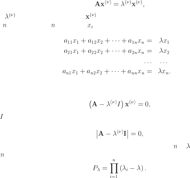
13.2 Eigenvalue problems

Let us consider the matrix A of dimension n. The eigenvalues of A is deﬁned through the matrix

equation

(13.1)

where

are the eigenvalues and the corresponding eigenvectors. This is equivalent to a

set of

equations with unknowns

W can rewrite eq (13.1) as

with being the unity matrix. This equation provides a solution to the problem if and only if the

determinant is zero, namely

which in turn means that the determinant is a polynomial of degree in and in general we will

have distinct zeros, viz.,

235

236 CHAPTER 13. EIGENSYSTEMS

Procedures based on these ideas con be used if only a small fraction of all eigenvalues and

eigenvectors are required, but the standard approach to solve eq. (13.1) is to perform a given

number of similarity transformations so as to render the original matrix

in: 1) a diagonal form

or: 2) as a tri-diagonal matrix which then can be be diagonalized by computational very effective

procedures.

The ﬁrst method leads us to e.g., Jacobi’s method whereas the second one is e.g., given by

Householder’s algorithm for tri-diagonal transformations. We will discuss both methods below.

13.2.1 Similarity transformations

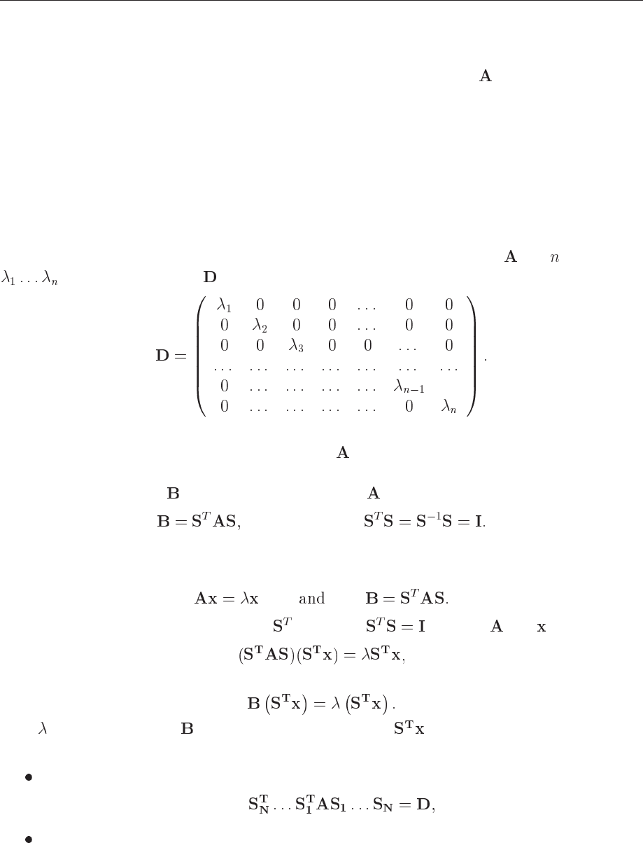
In the present discussion we assume that our matrix is real and symmetric, although it is rather

straightforward to extend it to the case of a hermitian matrix. The matrix

has eigenvalues

(distinct or not). Let be the diagonal matrix with the eigenvalues on the diagonal

(13.2)

The algorithm behind all current methods for obtaning eigenvalues is to perform a series of

similarity transformations on the original matrix to reduce it either into a diagonal form as

above or into a tri-diagonal form.

We say that a matrix

is a similarity transform of if

where (13.3)

The importance of a similarity transformation lies in the fact that the resulting matrix has the

same eigenvalues, but the eigenvectors are in general different. To prove this, suppose that

(13.4)

Multiply the ﬁrst equation on the left by

and insert between and . Then we get

(13.5)

which is the same as

(13.6)

Thus

is an eigenvalue of as well, but with eigenvector .

Now the basic philosophy is to

either apply subsequent similarity transformations so that

(13.7)

or apply subsequent similarity transformations so that A becomes tri-diagonal. Thereafter,

techniques for obtaining eigenvalues from tri-diagonal matrices can be used.

Let us look at the ﬁrst method, better known as Jacobi’s method.

13.2. EIGENVALUE PROBLEMS 237

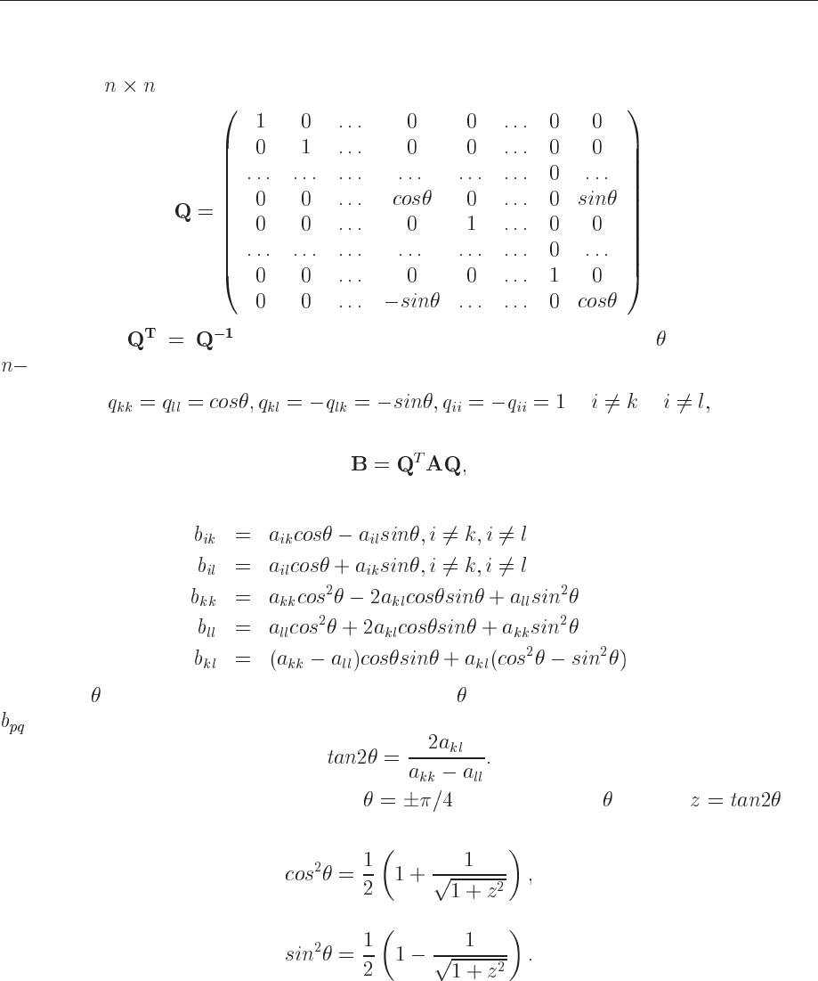
13.2.2 Jacobi’s method

Consider a (

) orthogonal transformation matrix

(13.8)

with property

. It performs a plane rotation around an angle in the Euclidean

dimensional space. It means that its matrix elements different from zero are given by

(13.9)

A similarity transformation

(13.10)

results in

(13.11)

The angle is arbitrary. Now the recipe is to choose so that all non-diagonal matrix elements

become zero which gives

(13.12)

If the denominator is zero, we can choose . Having deﬁned through , we

do not need to evaluate the other trigonometric functions, we can simply use relations like e.g.,

(13.13)

and

(13.14)

The algorithm is then quite simple. We perform a number of iterations untill the sum over the

squared non-diagonal matrix elements are less than a preﬁxed test (ideally equal zero). The

algorithm is more or less foolproof for all real symmetric matrices, but becomes much slower

than methods based on tri-diagonalization for large matrices. We do therefore not recommend

the use of this method for large scale problems. The philosophy however, performing a series of

similarity transformations pertains to all current models for matrix diagonalization.

238 CHAPTER 13. EIGENSYSTEMS

13.2.3 Diagonalizationthroughthe Householder’s methodfortri-diagonalization

In this case the energy diagonalization is performed in two steps: First, the matrix is transformed

into a tri-diagonal form by the Householder similarity transformation and second, the tri-diagonal

matrix is then diagonalized. The reason for this two-step process is that diagonalising a tri-

diagonal matrix is computational much faster then the corresponding diagonalization of a general

symmetric matrix. Let us discuss the two steps in more detail.

The Householder’s method for tri-diagonalization

The ﬁrst step consists in ﬁnding an orthogonal matrix

which is the product of orthog-

onal matrices

(13.15)

each of which successively transforms one row and one column of into the required tri-

diagonal form. Only transformations are required, since the last two elements are al-

ready in tri-diagonal form. In order to determine each

let us see what happens after the ﬁrst

multiplication, namely,

(13.16)

where the primed quantities represent a matrix of dimension which will subsequentely be

transformed by

. The factor is a possibly non-vanishing element. The next transformation

produced by has the same effect as but now on the submatirx only

(13.17)

Note that the effective size of the matrix on which we apply the transformation reduces for every

new step. In the previous Jacobi method each similarity transformation is performed on the full

size of the original matrix.

After a series of such transformations, we end with a set of diagonal matrix elements

(13.18)

and off-diagonal matrix elements

(13.19)