Hirsch M.J., Pardalos P.M., Murphey R. Dynamics of Information Systems: Theory and Applications
Подождите немного. Документ загружается.

266 P. DeLima et al.
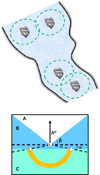
Fig. 13.8 Formation control
forsensorcoverage
optimization during transit
Fig. 13.9 Relative spatial
regions for mode transition
closest to the final destination select itself as the group leader, and leave the other to
position itself in formation behind the leader. However, if the poses of the two ships
do not match at the beginning of this task, the ASV nearest to the goal may need
to move further away to execute the desired maneuver, with each vessel obeying
the constraints of its physical dynamics and propulsion limitations. Furthermore, in
more realistic scenarios, such as the one visualized in Fig. 13.8 where the geome-
try of the waterway impedes the boats’ movements, predicting which specific craft
can achieve the shortest arrival time at the final destination in a distributed fashion
(in which information is only available locally and subject to change by other un-
controlled actors in the environment) is extremely difficult, and is subject to change
several times before the goal location is reached.
Consider the diagram shown in Fig. 13.9 in which the angle β is added to the
original configuration of Fig. 13.7, defining three separate regions (A, B, and C)
relative to the position and valid heading h
o
of the fleet leader. The task allocation
algorithm listed in Fig. 13.10 makes use of such regions to establish the negotiation
protocol that is employed by each and every member of the group operating in the
transit mode and having the same destination; the purpose of this procedure is to
select a single fleet leader in a distributed manner by iteratively converging to a
consensus. Note that the information required to execute this real-time negotiation

13.3 Decentralized Hierarchical Supervisor 267
1 if no leader is present
2 become leader
3 else
4 if there are multiple leaders that share the same destination
5 if this is the closest vehicle to the destination
6 become leader
7 else
8 become follower
9 else
10 if this vehicle is the current leader
11 and a follower is located within the region
A
12 become follower
13 else
14 if this vehicle is currently a follower
15 and it is located within the leader’s region
A
16 become leader
Fig. 13.10 Task allocation algorithm for the transit mode
protocol consists of the current position, pose, mode, and task of the neighboring
vessels.
Note that the evaluation of the other possible scenarios, such as the presence of
no leaders or of multiple leaders, is necessary for the successful resolution of the
transitory states that can be generated in the practical implementation of the nego-
tiation algorithm due to communication delays, for example. Furthermore, instead
of a direct threshold for the mode transitions in the final
else statement, the use of
the relative region A creates a hysteresis space which encompasses regions B and
a part of C, and prevents the emergence of oscillatory transitions between the ASV
roles due to the use of different trajectory generating strategies for each task.
13.3.2.2 Follower Trajectory Generating Algorithm
Having previously described the trajectory generating algorithm of the leader craft
as a simplification of the search procedure described in Sect. 13.3.1, here, we in-
troduce a trajectory generation algorithm for the follower craft. As previously men-
tioned, as a follower, an ASV must achieve both the primary goal of arriving at
the destination, and the secondary goal of maximizing the overall sensor coverage
of the entire group. While the process of evaluating the desired heading h remains
the same (see Sect. 13.3.1), the algorithm for generating the h is modified to better
fit the priorities of a follower unit. For these boats, the desired heading h is a nor-
malization of the sum of the two vectors: the tracking vector t, and the positioning
vector p, as illustrated in Fig. 13.11. The purpose of the tracking vector t is to ensure
that the followers maintain their relative positions with respect to the current leader,
hence t is defined along the same direction as the valid heading h
o
of the leader.
268 P. DeLima et al.
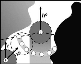
Fig. 13.11 Example scenario for the generation of the tracking vector t, and the positioning vec-
tor p for the determination of the desired heading h of a follower craft. Shaded areas represent
regions that were already scanned by the ASVs, while the black area on the right side of the image
represents a nontraversable zone
The positioning vector p guides the craft to a point around the leader craft within
the semi-arch of a radius equal to twice the sensor range of the vehicles, so that
the joint area coverage of the group is maximized. The direction of p is defined in
terms of the current position of the follower, and the position along the previously
computed semi-arch around the leading vessel that is both feasible, and results in the
greatest gain for the combined sensor coverage of the fleet, taking into consideration
the traversability map and the mission’s coverage status map [7]. This position is
selected from a set of finite, equally spaced candidates along the formation semi-
arch, as in the example configuration depicted in Fig. 13.11. While the direction
vector t is a unit vector, the norm of vector p is equal to the distance between the
current position of the follower craft and the selected position along the formation
semi-arch. Constructed in this manner, the resulting desired heading h is dominated
by p at greater distances, but as the desired position is approached, the influence of
t increases gradually, allowing the vehicles to maintain formation. Once a desired
heading h is established, it evaluates h
before generating the craft’s final navigation
vector h
o
. Recall that the obstacle avoidance routine, which constantly operates at a
lower control level, will prevent any collision-prone h
o
from being undertaken by a
vehicle.
We should note that in order to generate the necessary formations in all of the
potential collaborative transit scenarios, control of the heading alone is insufficient.
In order to “catch up” with a distant leader, or to yield when moving ahead of the de-
sired relative position, it is also necessary to implement some form of speed control.
For this purpose, we developed a new speed control function shown in Fig. 13.12,
where fixed speed-differential values are assigned based on the relative positions
of the followers with respect to the transit leader. The speed control map is tuned
to fit the vehicle’s dynamic constraints, particularly with respect to the maximum
achievable and minimum effective speeds. In all cases, however, it is important that
the final curves traced by the craft’s control algorithm through the state space be
smooth and at least piece-wise continuous. To fulfill both of these requirements, the
13.3 Decentralized Hierarchical Supervisor 269
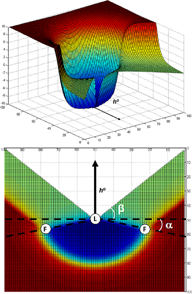
Fig. 13.12 Sample speed adjustment maps shown in 3D and 2D perspectives. White circles in-
dicate task leader location (L) and optimal follower locations (F); the map orientation vector h
o
indicates the leader’s current valid heading. Bright shaded areas represent a neutral relative speed
and serve as follower attractors, while the darker area in the circular section in the center is related
to slower speeds, and the darker area outside corresponds to faster speeds

270 P. DeLima et al.
generated speed map was constructed from sigmoidal primitives of the form:
S =A
x
√
1 +x
2
where S is the speed differential over the vehicle’s standard cruise speed, A is the
amplitude of the maximum allowed speed differential (A = 10 m/s in the example
shown in Fig. 13.12), and x is the distance to a relative point in the speed map with
respect to the leader’s location (a valid heading is chosen to generate the desired
shape).
From the speed map’s three dimensional representation (Fig. 13.12, left), observe
that in the formation semi-arch region, the speed differential is zero, and since the
heading of the follower at these locations matches that of the leader (i.e., p has a zero
norm), these areas represent followers’ convergence points. The speed-differential
map is not defined in region A because as soon as a follower moves into this po-
sition, the task assignment algorithm (see Sect. 13.3.2.1) will select it as the new
leader, and the ASV will not alter its speed from the standard cruise value.
13.4 Simulation Results
To demonstrate the benefit of cooperation that can be realized with the proposed
search and transit task algorithms, we simulated missions using both cooperating
and noncooperating ASVs. The simulated mission conducted under both configura-
tions consisted of searching two separate locations within a designated mission area.
These two search regions were located in different portions of the mission area, sep-
arated by a “river” (i.e., a narrow traversable channel such that no single constant
heading can be used to navigate from one search area to another).
The mission began with the two ASVs at different traversable locations selected
at random within the south-east (SE) search area. After 20% of the total mission time
had elapsed, both ASVs were instructed to perform the search of the north-west area,
followed by another search command after 65% of the mission time, indicating once
more the need to search the original SE search area. Figure 13.13 shows an example
trace of the cooperative ASV simulation in which the search begins at the bottom-
right corner, then switches to the second search area at the top-left corner of the
mission area.
In order to generate results for the same mission operating without cooperation
among ASVs, we eliminated the ship-to-ship communication in the second set of
simulations. During the search task, a lack of communication results in each unit
not being aware of the area covered by the sensors of the other, therefore causing
each craft to compute its movements based solely on the information contained in
the individual on-board dynamic coverage map. During the transit task, since each
vehicle lacks the knowledge of the common destination it shares with its neighbor,
both assume the role of leaders, and proceed to minimize the arrival time without
attempting to increase the joint sensor coverage. An example of a run without the
cooperation between the craft can be seen in Fig. 13.14.
13.4 Simulation Results 271
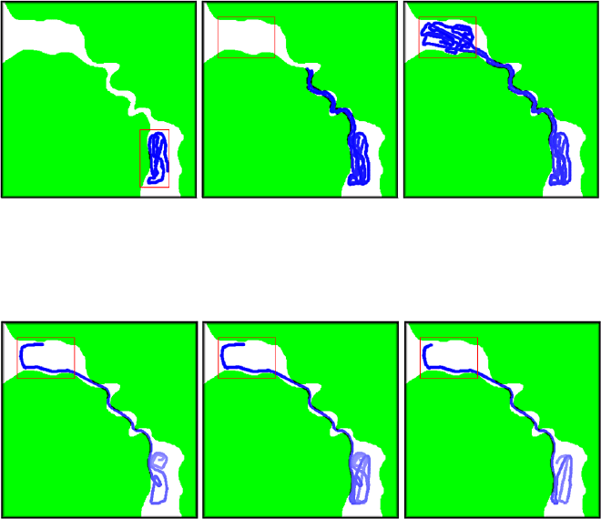
Fig. 13.13 Visualization of the multi-objective mission involving the collaborative search of a des-
ignated area in the SE corner of the map (left) by two autonomous ASVs, followed by a search-in–
transit while navigating a river channel in formation (middle), and resumption of the search within
the NW zone (right)
Fig. 13.14 Visualization of the multi-objective mission without communication between ASVs.
The map on the left shows the self-perceived coverage of the first ASV. The map on the right
displays the same content from the perspective of the second ASV. The map in the center shows
the combined effect on sensor coverage from both ASVs, generated after the end of the mission by
a global observer
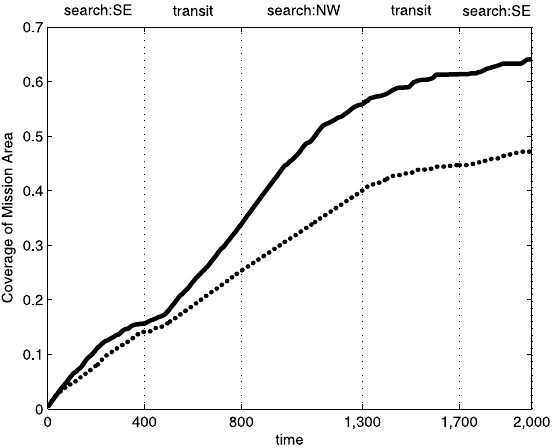
To generate statistically accurate results, a total of 20 empirical experiments were
performed for each mission scenario. The comparison between the average coverage
of the entire search region (i.e., the two search areas and the river channel connect-
ing them) over time in the two scenarios is plotted in Fig. 13.15. Note that a marked
improvement in the search coverage due to the cooperation between the two boats
can be seen during the initial moments of the simulation, when the mission goal
is to search the SE area. The difference in slopes of the two curves increases as
the cooperative behavior exhibited by the craft that assumes the follower role dur-
ing transit provides additional coverage in the region between the two search areas.
A pronounced increase in the sensor coverage performance can also be seen dur-
ing the search performed in the NW search area, where the absence of cooperation
between the ASVs becomes particularly detrimental. This result is due in part to
the fact that the lack of communication caused the craft to use nearby entry points
into the search area after emerging from the river channel, which subsequently leads
to highly similar navigation decisions (i.e., the two craft end up covering the same
272 P. DeLima et al.
Fig. 13.15 Comparison of the coverage of the total mission area achieved during each of the
search and transit intervals of the mission for the cooperative (solid) and independent (dashed)
scenarios
regions). On average, within the parameters of the constructed mission, the sensor
coverage of the SE area increased by 17.53% when cooperation was allowed, while
the much larger gain of 48.89% was realized in the NW area. During the transit
from the SE area to the NW area, the execution of the proposed cooperative transit
algorithm resulted in a 47.06% increase in the coverage of the region connecting
the two search areas. Using the Wilcoxon rank sum test [3], we found that the task
performance improvements achieved by the cooperative controller are statistically
significant from the noncooperative version (p =0.01).
13.5 Conclusion and Future Work
In this chapter, we presented a novel decentralized hierarchical supervisor archi-
tecture for unmanned surface vehicles composed of four layers for mode selection,
task allocation, trajectory generation, and tracking control. For vehicles deployed
on surveillance missions involving multiple disjoint areas, we have developed the
modes of surveillance and transit, and described the autonomous algorithms that
compose each of the corresponding supervisor layers. Simulation results from test-
ing the application of the proposed architecture revealed statistically significant ben-
efits of the cooperative control algorithm over conventional, independent approaches
in terms of increasing the performance of concurrent search and transit objectives
References 273
with only a modest increase in the ASVs’ on-board hardware and communication
requirements.
Advances outlined here comprise a part of a much larger research effort concern-
ing the technological gap between current state-of-the-art manned and unmanned
systems. The long-term goal of this work is to construct a comprehensive frame-
work for analysis and development of such collaborative technologies, and the over-
all feasibility of our approach for solving real-world problems is evident from the
numerous successful outcomes we achieved with multiple autonomous platforms on
a set of nontrivial, complex, challenging tasks [10].
References
1. Benjamin, M., Curcio, J., Leonard, J., Newman, P.: A method for protocol-based collision
avoidance between autonomous marine surface craft. J. Field Robotics 23(5) (2006)
2. DeLima, P., Pack, D.: Toward developing an optimal cooperative search algorithm for multiple
unmanned aerial vehicles. In: Proceedings of the International Symposium on Collaborative
Technologies and Systems (CTS-08), pp. 506–512, May 2008
3. Gibbons, J.D.: Nonparametric Statistical Inference. Marcel Dekker, New York (1985)
4. Matos, A., Cruz, N.: Coordinated operation of autonomous underwater and surface vehicles.
In: Proceedings of the Oceans 2007, pp. 1–6, October 2007
5. Pack, D., York, G.: Developing a control architecture for multiple unmanned aerial vehicles
to search and localize RF time-varying mobile targets: part I. In: Proceedings of the IEEE
International Conference on Robotics and Automation, pp. 3965–3970, April 2005
6. Pack, D., DeLima, P., Toussaint, G., York, G.: Cooperative control of UAVs for localization of
intermittently emitting mobile targets. IEEE Trans. Syst. Man Cybern. Part B, Cybern. 39(4),
959–970 (2009)
7. Plett, G., DeLima, P., Pack, D.: Target localization using multiple UAVs with sensor fusion
via Sigma-Point Kalman filtering. In: Proceedings of the 2007 AIAA (2007)
8. Plett, G., Zarzhitsky, D., Pack, D.: Out-of-order Sigma-Point Kalman filtering for target local-
ization using cooperating unmanned aerial vehicles. In: Hirsch, M.J., Pardalos, P.M., Murphey,
R., Grundel, D. (eds.) Advances in Cooperative Control and Optimization. Lecture Notes in
Control and Information Sciences, vol. 369, pp. 22–44 (2007)
9. Willcox, S., Goldberg, D., Vaganay, J., Curcio, J.: Multi-vehicle cooperative navigation and
autonomy with the bluefin CADRE system. In: Proceedings of the International Federation of
Automatic Control Conference (IFAC-06), September 2006
10. Zarzhitsky, D., Schlegel, M., Decker, A., Pack, D.: An event-driven software architecture for
multiple unmanned aerial vehicles to cooperatively locate mobile targets. In: Hirsch, M.J.,
Commander, C., Pardalos, P.M., Murphey, R. (eds.) Optimization and Cooperative Control
Strategies. Lecture Notes in Control and Information Sciences, vol. 381, pp. 299–318 (2009)

Chapter 14
A Connectivity Reduction Strategy
for Multi-agent Systems
Xiaojun Geng and David Jeffcoat
Summary This paper considers the connectivity reduction of multi-agent systems
which are represented with directed graphs. A simple distributed algorithm is pre-
sented for each agent to independently remove some of its incoming links based
on only the local information of its neighbors. The algorithm results in an infor-
mation graph with sparser connections. The goal is to reduce computational effort
associated with communication while still maintaining overall system performance.
The main contribution of this paper is a distributed algorithm that can, under certain
conditions, find and remove redundant edges in a directed graph using only local
information.
14.1 Introduction
Groups of multiple agents have been studied with the aid of algebraic graph the-
ory, for example, in [2, 4, 7, 8, 10, 11], and [5]. Directed or undirected, weighted
or unweighted graphs are used to characterize a network of multiple agents, in
which agents are represented by vertices of a graph and information interactions
by arcs/edges. Once a graph is constructed for the networked agents, decentralized
control laws are applied to drive the behavior of each agent using only information
available to that agent. This information comes from its own sensing devices or from
other agents through communications.
Generally, more local information available to each individual agent results in
better performance for the overall group. The second smallest eigenvalue of the
Laplacian matrix, also called the algebraic connectivity of the graph, has been used
X. Geng (
)
California State University, 18111 Nordhoff St., Northridge, CA 91330, USA
e-mail: xjgeng@csun.edu
D. Jeffcoat
Air Force Research Laboratory, Eglin AFB, FL 32542, USA
e-mail: david.jeffcoat@eglin.af.mil
M.J. Hirsch et al. (eds.), Dynamics of Information Systems,
Springer Optimization and Its Applications 40, DOI 10.1007/978-1-4419-5689-7_14,
© Springer Science+Business Media, LLC 2010
275