Hirsch M., Smale S., Devaney R., Differential Equations, Dynamical Systems, and an Introduction to Chaos

Подождите немного. Документ загружается.

16 Chapter 1 First-Order Equations

8. Consider the differential equation x



= x − x

− b sin(2πt ) where |b| is

small. What can you say about solutions of this equation? Are there any

periodic solutions?

9. Experimentally, what happens as |b| increases? Do you observe any

bifurcations? Explain what you observe.

EXERCISES

1. Find the general solution of the differential equation x



= ax + 3 where

a is a parameter. What are the equilibrium points for this equation? For

which values of a are the equilibria sinks? For which are they sources?

2. For each of the following differential equations, ﬁnd all equilibrium

solutions and determine if they are sinks, sources, or neither. Also, sketch

the phase line.

(a) x



= x

− 3x

(b) x



= x

− x



= cos x

(d) x



= sin

(e) x



=|1 − x

3. Each of the following families of differential equations depends on a

parameter a. Sketch the corresponding bifurcation diagrams.

(a) x



= x

− ax

(b) x



= x

− ax



= x

− x + a

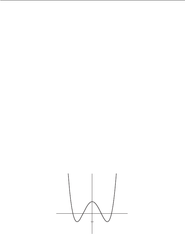
4. Consider the function f (x) whose graph is displayed in Figure 1.12.

f(x)

Figure 1.12 The graph of the

function f.

Exercises 17

(a) Sketch the phase line corresponding to the differential equation x



f (x).

(b) Let g

(x) = f (x)+a. Sketch the bifurcation diagram corresponding

to the family of differential equations x



= g

(x).

5. Consider the family of differential equations



= ax + sin x

where a is a parameter.

(a) Sketch the phase line when a = 0.

(b) Use the graphs of ax and sin x to determine the qualitative behavior

of all of the bifurcations that occur as a increases from −1to1.

equations.

6. Find the general solution of the logistic differential equation with

constant harvesting



= x(1 − x) − h

for all values of the parameter h>0.

7. Consider the nonautonomous differential equation





x − 4ift<5

2 − x if t ≥ 5

(a) Find a solution of this equation satisfying x(0) = 4. Describe the

qualitative behavior of this solution.

(b) Find a solution of this equation satisfying x(0) = 3. Describe the

qualitative behavior of this solution.

t →∞.

8. Consider a ﬁrst-order linear equation of the form x



= ax + f (t ) where

a ∈

R. Let y(t ) be any solution of this equation. Prove that the general

solution is y(t ) + c exp(at ) where c ∈

R is arbitrary.

9. Consider a ﬁrst-order, linear, nonautonomous equation of the form



(t) = a(t)x.

(a) Find a formula involving integrals for the solution of this system.

(b) Prove that your formula gives the general solution of this system.

18 Chapter 1 First-Order Equations

10. Consider the differential equation x



= x + cos t.

(a) Find the general solution of this equation.

(b) Prove that there is a unique periodic solution for this equation.

tion and use this to verify again that there is a unique periodic

solution.

11. First-order differential equations need not have solutions that are deﬁned

for all times.

(a) Find the general solution of the equation x



= x

(b) Discuss the domains over which each solution is deﬁned.

satisfying x(0) = 0 is deﬁned only for −1 <t<1.

12. First-order differential equations need not have unique solutions satis-

fying a given initial condition.

(a) Prove that there are inﬁnitely many different solutions of the

differential equations x



= x

1/3

satisfying x(0) = 0.

(b) Discuss the corresponding situation that occurs for x



= x/t ,

x(0) = x



= x/t

, x(0) = 0.

13. Let x



= f (x) be an autonomous ﬁrst-order differential equation with

an equilibrium point at x

(a) Suppose f



) = 0. What can you say about the behavior of

solutions near x

? Give examples.

(b) Suppose f



) = 0 and f



) = 0. What can you now say?



) = f



) = 0 but f



) = 0. What can you now

say?

14. Consider the ﬁrst-order nonautonomous equation x



= p(t)x where

p(t ) is differentiable and periodic with period T . Prove that all solutions

of this equation are periodic with period T if and only if



p(s) ds = 0.

15. Consider the differential equation x



= f (t , x) where f (t , x) is continu-

ously differentiable in t and x. Suppose that

f (t + T , x) = f (t , x)

Exercises 19

for all t . Suppose there are constants p, q such that

f (t, p) > 0, f (t , q) < 0

for all t . Prove that there is a periodic solution x(t ) for this equation with

p<x(0) <q.

16. Consider the differential equation x



= x

− 1 − cos(t). What can be

said about the existence of periodic solutions for this equation?

This Page Intentionally Left Blank

Planar Linear Systems

In this chapter we begin the study of systems of differential equations. A system

of differential equations is a collection of n interrelated differential equations

of the form



= f

(t, x

, x

, ..., x

)



= f

(t, x

, x

, ..., x

)



= f

(t, x

, x

, ..., x

Here the functions f

are real-valued functions of the n +1 variables x

, x

, ...,

, and t . Unless otherwise speciﬁed, we will always assume that the f

are C

∞

functions. This means that the partial derivatives of all orders of the f

exist

and are continuous.

To simplify notation, we will use vector notation:

X =

⎛

⎜

⎝

⎞

⎟

⎠

We often write the vector X as (x

, ..., x

) to save space.

22 Chapter 2 Planar Linear Systems

Our system may then be written more concisely as



= F(t, X)

where

F(t , X) =

⎛

⎜

⎝

(t, x

, ..., x

)

(t, x

, ..., x

)

⎞

⎟

⎠

A solution of this system is then a function of the form X(t ) =

(t), ..., x

(t)) that satisﬁes the equation, so that



(t) = F(t , X(t))

where X



(t) = (x



(t), ..., x



(t)). Of course, at this stage, we have no guarantee

that there is such a solution, but we will begin to discuss this complicated

question in Section 2.7.

The system of equations is called autonomous if none of the f

depends on

t, so the system becomes X



= F(X). For most of the rest of this book we will

be concerned with autonomous systems.

In analogy with ﬁrst-order differential equations, a vector X

for which

F(X

) = 0 is called an equilibrium point for the system. An equilibrium point

corresponds to a constant solution X(t) ≡ X

of the system as before.

Just to set some notation once and for all, we will always denote real variables

by lowercase letters such as x, y, x

, x

, t , and so forth. Real-valued functions

will also be written in lowercase such as f (x, y)orf

, ..., x

, t ). We will

reserve capital letters for vectors such as X = (x

, ..., x

), or for vector-valued

functions such as

F(x, y) = (f (x, y), g (x, y))

H(x

, ..., x

) =

⎛

⎜

⎝

, ..., x

)

, ..., x

)

⎞

⎟

⎠

We will denote n-dimensional Euclidean space by

, so that R

consists of

all vectors of the form X = (x

, ..., x

2.1 Second-Order Differential Equations 23

2.1 Second-Order Differential Equations

Many of the most important differential equations encountered in science

and engineering are second-order differential equations. These are differential

equations of the form



= f (t , x, x



Important examples of second-order equations include Newton’s equation



= f (x),

the equation for an RLC circuit in electrical engineering

LCx



+ RCx



+ x = v(t),

and the mainstay of most elementary differential equations courses, the forced

harmonic oscillator



+ bx



+ kx = f (t ).

We will discuss these and more complicated relatives of these equations at

length as we go along. First, however, we note that these equations are a

special subclass of two-dimensional systems of differential equations that are

deﬁned by simply introducing a second variable y = x



For example, consider a second-order constant coefﬁcient equation of the

form



+ ax



+ bx = 0.

If we let y = x



, then we may rewrite this equation as a system of ﬁrst-order

equations



= y



=−bx − ay.

Any second-order equation can be handled in a similar manner. Thus, for the

remainder of this book, we will deal primarily with systems of equations.

24 Chapter 2 Planar Linear Systems

2.2 Planar Systems

For the remainder of this chapter we will deal with autonomous systems in

, which we will write in the form



= f (x, y)



= g (x, y)

thus eliminating the annoying subscripts on the functions and variables. As

above, we often use the abbreviated notation X



= F(X) where X = (x, y)

and F (X) = F(x, y) = (f (x, y), g (x, y)).

In analogy with the slope ﬁelds of Chapter 1, we regard the right-hand side

of this equation as deﬁning a vector ﬁeld on

. That is, we think of F(x, y)

as representing a vector whose x- and y-components are f (x, y) and g (x, y),

respectively. We visualize this vector as being based at the point (x, y). For

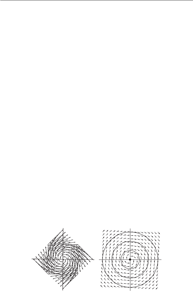
example, the vector ﬁeld associated to the system



= y



=−x

is displayed in Figure 2.1. Note that, in this case, many of the vectors overlap,

making the pattern difﬁcult to visualize. For this reason, we always draw a

direction ﬁeld instead, which consists of scaled versions of the vectors.

A solution of this system should now be thought of as a parameterized curve

in the plane of the form (x(t ), y(t )) such that, for each t , the tangent vector at

the point (x(t), y(t )) is F(x(t ), y(t )). That is, the solution curve (x(t ), y(t ))

winds its way through the plane always tangent to the given vector F(x(t ), y(t ))

based at (x(t ), y(t )).

Figure 2.1 The vector field, direction field, and

several solutions for the system x



= y, y



=–x.

2.2 Planar Systems 25

Example. The curve



x(t )

y(t)





a sin t

a cos t



for any a ∈

R is a solution of the system



= y



=−x

since



(t) = a cos t = y(t )



(t) =−a sin t =−x(t )

as required by the differential equation. These curves deﬁne circles of radius

|a| in the plane that are traversed in the clockwise direction as t increases.

When a = 0, the solutions are the constant functions x(t ) ≡ 0 ≡ y(t).



Note that this example is equivalent to the second-order differential equa-

tion x



=−x by simply introducing the second variable y = x



. This is an

example of a linear second-order differential equation, which, in more general

form, can be written

a(t )x



+ b(t)x



+ c(t )x = f (t ).

An important special case of this is the linear, constant coefﬁcient equation



+ bx



+ cx = f (t ),

which we write as a system as



= y



=−

x −

y +

f (t)

An even more special case is the homogeneous equation in which f (t ) ≡ 0.

Example. One of the simplest yet most important second-order, linear, con-

stant coefﬁcient differential equations is the equation for a harmonic oscillator.

This equation models the motion of a mass attached to a spring. The spring

is attached to a vertical wall and the mass is allowed to slide along a hori-

zontal track. We let x denote the displacement of the mass from its natural