Hirsch M., Smale S., Devaney R., Differential Equations, Dynamical Systems, and an Introduction to Chaos

Подождите немного. Документ загружается.

6 Chapter 1 First-Order Equations

x⫽1

x⫽0

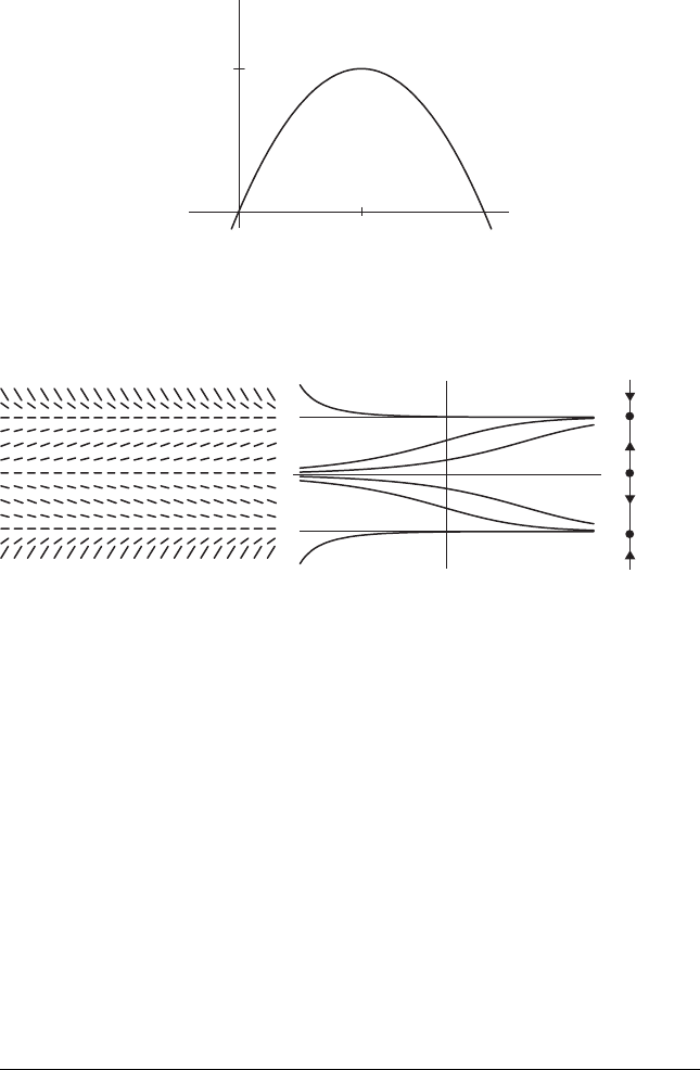
Figure 1.3 The slope field, solution graphs, and phase line for



= ax(1 – x).

To get a qualitative feeling for the behavior of solutions, we sketch the

slope ﬁeld for this equation. The right-hand side of the differential equation

determines the slope of the graph of any solution at each time t . Hence we

may plot little slope lines in the tx–plane as in Figure 1.3, with the slope of the

line at (t , x) given by the quantity ax(1 − x). Our solutions must therefore

have graphs that are everywhere tangent to this slope ﬁeld. From these graphs,

we see immediately that, in agreement with our assumptions, all solutions

for which x(0) > 0 tend to the ideal population x(t ) ≡ 1. For x(0) < 0,

solutions tend to −∞, although these solutions are irrelevant in the context

of a population model.

Note that we can also read this behavior from the graph of the function

(x) = ax(1 − x). This graph, displayed in Figure 1.4, crosses the x-axis at

the two points x = 0 and x = 1, so these represent our equilibrium points.

When 0 <x<1, we have f (x) > 0. Hence slopes are positive at any (t , x)

with 0 <x<1, and so solutions must increase in this region. When x<0or

x>1, we have f (x) < 0 and so solutions must decrease, as we see in both the

solution graphs and the phase lines in Figure 1.3.

We may read off the fact that x = 0 is a source and x = 1 is a sink from

the graph of f in similar fashion. Near 0, we have f (x) > 0ifx>0, so slopes

are positive and solutions increase, but if x<0, then f (x) < 0, so slopes are

negative and solutions decrease. Thus nearby solutions move away from 0 and

so 0 is a source. Similarly, 1 is a sink.

We may also determine this information analytically. We have f



(x) =

a − 2ax so that f



(0) = a>0 and f



(1) =−a<0. Since f



(0) > 0, slopes

must increase through the value 0 as x passes through 0. That is, slopes are

negative below x = 0 and positive above x = 0. Hence solutions must tend

away from x = 0. In similar fashion, f



(1) < 0 forces solutions to tend toward

x = 1, making this equilibrium point a sink. We will encounter many such

“derivative tests” like this that predict the qualitative behavior near equilibria

in subsequent chapters.

1.3 Constant Harvesting and Bifurcations 7

0.8

0.5 1

Figure 1.4 The graph of the

function f (x)=ax(1 – x) with

a = 3.2.

x⫽1

x⫽⫺1

x⫽0

Figure 1.5 The slope field, solution graphs, and phase line for x



= x – x

Example. As a further illustration of these qualitative ideas, consider the

differential equation



= g (x) = x − x

There are three equilibrium points, at x = 0, ±1. Since g



(x) = 1 − 3x

,we

have g



(0) = 1, so the equilibrium point 0 is a source. Also, g



(±1) =−2, so

the equilibrium points at ±1 are both sinks. Between these equilibria, the sign

of the slope ﬁeld of this equation is nonzero. From this information we can

immediately display the phase line, which is shown in Figure 1.5.



1.3 Constant Harvesting and

Bifurcations

Now let’s modify the logistic model to take into account harvesting of the pop-

ulation. Suppose that the population obeys the logistic assumptions with the

8 Chapter 1 First-Order Equations

0.5

h⬍1/

h⫽1/

h⬎1/

(x)

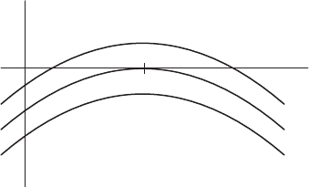
Figure 1.6 The graphs of the function

(x)=x(1 – x)–h.

parameter a = 1, but is also harvested at the constant rate h. The differential

equation becomes



= x(1 − x) − h

where h ≥ 0 is a new parameter.

Rather than solving this equation explicitly (which can be done — see

Exercise 6 at the end of this chapter), we use the graphs of the functions

(x) = x(1 − x) − h

to “read off ” the qualitative behavior of solutions. In Figure 1.6 we display

the graph of f

in three different cases: 0 <h<1/4, h = 1/4, and h>1/4.

It is straightforward to check that f

has two roots when 0 ≤ h<1/4, one

root when h = 1/4, and no roots if h>1/4, as illustrated in the graphs. As a

consequence, the differential equation has two equilibrium points x



and x

with 0 ≤ x



when 0 <h<1/4. It is also easy to check that f





) > 0, so

that x



is a source, and f



) < 0 so that x

is a sink.

As h passes through h = 1/4, we encounter another example of a bifurcation.

The two equilibria x



and x

coalesce as h increases through 1/4 and then

disappear when h>1/4. Moreover, when h>1/4, we have f

(x) < 0 for all

x. Mathematically, this means that all solutions of the differential equation

decrease to −∞ as time goes on.

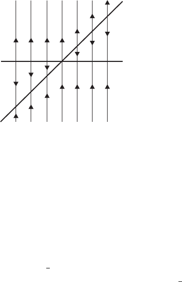
We record this visually in the bifurcation diagram. In this diagram we plot

the parameter h horizontally. Over each h-value we plot the corresponding

phase line. The curve in this picture represents the equilibrium points for each

value of h. This gives another view of the sink and source merging into a

single equilibrium point and then disappearing as h passes through 1/4 (see

Figure 1.7).

Ecologically, this bifurcation corresponds to a disaster for the species under

study. For rates of harvesting 1/4 or lower, the population persists, provided

1.4 Periodic Harvesting and Periodic Solutions 9

1/4

Figure 1.7 The bifurcation diagram for

(x)=x(1 – x)–h.

the initial population is sufﬁciently large (x(0) ≥ x



). But a very small change

in the rate of harvesting when h = 1/4 leads to a major change in the fate of

the population: At any rate of harvesting h>1/4, the species becomes extinct.

This phenomenon highlights the importance of detecting bifurcations in

families of differential equations, a procedure that we will encounter many

times in later chapters. We should also mention that, despite the simplicity of

this population model, the prediction that small changes in harvesting rates

can lead to disastrous changes in population has been observed many times in

real situations on earth.

Example. As another example of a bifurcation, consider the family of

differential equations



= g

(x) = x

− ax = x(x − a)

which depends on a parameter a. The equilibrium points are given by x = 0

and x = a. We compute g



(0) =−a, so 0 is a sink if a>0 and a source if

a<0. Similarly, g



(a) = a,sox = a is a sink if a<0 and a source if a>0.

We have a bifurcation at a = 0 since there is only one equilibrium point when

a = 0. Moreover, the equilibrium point at 0 changes from a source to a sink

as a increases through 0. Similarly, the equilibrium at x = a changes from a

sink to a source as a passes through 0. The bifurcation diagram for this family

is depicted in Figure 1.8.



1.4 Periodic Harvesting and

Periodic Solutions

Now let’s change our assumptions about the logistic model to reﬂect the

fact that harvesting does not always occur at a constant rate. For example,

10 Chapter 1 First-Order Equations

x⫽a

Figure 1.8 The bifurcation

diagram for x



= x

– ax.

populations of many species of ﬁsh are harvested at a higher rate in warmer

seasons than in colder months. So we assume that the population is harvested

at a periodic rate. One such model is then



= f (t , x) = ax(1 − x) − h(1 + sin(2πt ))

where again a and h are positive parameters. Thus the harvesting reaches a

maximum rate −2h at time t =

+n where n is an integer (representing the

year), and the harvesting reaches its minimum value 0 when t =

+n, exactly

one-half year later. Note that this differential equation now depends explicitly

on time; this is an example of a nonautonomous differential equation. As in

the autonomous case, a solution x(t ) of this equation must satisfy x



(t) =

f (t, x(t)) for all t . Also, this differential equation is no longer separable, so we

cannot generate an analytic formula for its solution using the usual methods

from calculus. Thus we are forced to take a more qualitative approach.

To describe the fate of the population in this case, we ﬁrst note that the right-

hand side of the differential equation is periodic with period 1 in the time

variable. That is, f (t + 1, x) = f (t , x). This fact simpliﬁes somewhat the

problem of ﬁnding solutions. Suppose that we know the solution of all initial

value problems, not for all times, but only for 0 ≤ t ≤ 1. Then in fact we

know the solutions for all time. For example, suppose x

(t) is the solution that

is deﬁned for 0 ≤ t ≤ 1 and satisﬁes x

(0) = x

. Suppose that x

(t)isthe

solution that satisﬁes x

(0) = x

(1). Then we may extend the solution x

deﬁning x

(t + 1) = x

(t) for 0 ≤ t ≤ 1. The extended function is a solution

since we have



(t + 1) = x



(t) = f (t , x

(t))

= f (t + 1, x

(t + 1)).

1.4 Periodic Harvesting and Periodic Solutions

Figure 1.9 The slope field for f (x)=

x (1 – x)–h (1 + sin (2πt)).

Thus if we know the behavior of all solutions in the interval 0 ≤ t ≤ 1, then

we can extrapolate in similar fashion to all time intervals and thereby know

the behavior of solutions for all time.

Secondly, suppose that we know the value at time t = 1 of the solution

satisfying any initial condition x(0) = x

. Then, to each such initial condition

, we can associate the value x(1) of the solution x(t ) that satisﬁes x(0) = x

This gives us a function p(x

) = x(1). If we compose this function with itself,

we derive the value of the solution through x

at time 2; that is, p(p(x

)) =

x(2). If we compose this function with itself n times, then we can compute

the value of the solution curve at time n and hence we know the fate of the

solution curve.

The function p is called a Poincaré map for this differential equation. Having

such a function allows us to move from the realm of continuous dynamical

systems (differential equations) to the often easier-to-understand realm of

discrete dynamical systems (iterated functions). For example, suppose that

we know that p(x

) = x

for some initial condition x

. That is, x

is a ﬁxed

point for the function p. Then from our previous observations, we know that

x(n) = x

for each integer n. Moreover, for each time t with 0 <t<1, we

also have x(t) = x(t + 1) and hence x(t + n) = x(t ) for each integer n.

That is, the solution satisfying the initial condition x(0) = x

is a periodic

function of t with period 1. Such solutions are called periodic solutions of the

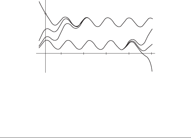
differential equation. In Figure 1.10, we have displayed several solutions of the

logistic equation with periodic harvesting. Note that the solution satisfying

the initial condition x(0) = x

is a periodic solution, and we have x

p(x

) = p(p(x

)) .... Similarly, the solution satisfying the initial condition

x(0) =ˆx

also appears to be a periodic solution, so we should have p(ˆx

) =ˆx

Unfortunately, it is usually the case that computing a Poincaré map for a

differential equation is impossible, but for the logistic equation with periodic

harvesting we get lucky.

12 Chapter 1 First-Order Equations

t⫽0

x(1)⫽p(x

) x(2)⫽p(p(x

))

t⫽1 t⫽2

∧

Figure 1.10 The Poincaré map for x



=5x(1 – x)–

0.8(1 + sin (2πt)).

1.5 Computing the Poincaré Map

Before computing the Poincaré map for this equation, we introduce some

important terminology. To emphasize the dependence of a solution on the

initial value x

, we will denote the corresponding solution by φ(t , x

). This

function φ :

R × R → R is called the ﬂow associated to the differential

equation. If we hold the variable x

ﬁxed, then the function

t → φ(t, x

)

is just an alternative expression for the solution of the differential equation

satisfying the initial condition x

. Sometimes we write this function as φ

Example. For our ﬁrst example, x



= ax, the ﬂow is given by

φ(t , x

) = x

For the logistic equation (without harvesting), the ﬂow is

φ(t , x

) =

x(0)e

1 − x(0) + x(0)e

Now we return to the logistic differential equation with periodic harvesting



= f (t , x) = ax(1 − x) − h(1 + sin(2πt )).

1.5 Computing the Poincaré Map 13

The solution satisfying the initial condition x(0) = x

is given by t → φ(t , x

While we do not have a formula for this expression, we do know that, by the

fundamental theorem of calculus, this solution satisﬁes

φ(t , x

) = x



f (s, φ(s, x

)) ds

since

∂φ

∂t

(t, x

) = f (t , φ(t , x

))

and φ(0, x

) = x

If we differentiate this solution with respect to x

, we obtain, using the chain

rule:

∂φ

∂x

(t, x

) = 1 +



∂f

∂x

(s, φ(s, x

)) ·

∂φ

∂x

(s, x

) ds.

Now let

z(t ) =

∂φ

∂x

(t, x

Note that

z(0) =

∂φ

∂x

(0, x

) = 1.

Differentiating z with respect to t ,weﬁnd



(t) =

∂f

∂x

(t, φ(t, x

)) ·

∂φ

∂x

(t, x

)

∂f

∂x

(t, φ(t, x

)) · z(t ).

Again, we do not know φ(t , x

) explicitly, but this equation does tell us that

z(t ) solves the differential equation



(t) =

∂f

∂x

(t, φ(t, x

)) z(t )

with z(0) = 1. Consequently, via separation of variables, we may compute

that the solution of this equation is

z(t ) = exp



∂f

∂x

(s, φ(s, x

)) ds

14 Chapter 1 First-Order Equations

and so we ﬁnd

∂φ

∂x

(1, x

) = exp



∂f

∂x

(s, φ(s, x

)) ds.

Since p(x

) = φ(1, x

), we have determined the derivative p



)ofthe

Poincaré map. Note that p



) > 0. Therefore p is an increasing function.

Differentiating once more, we ﬁnd



) = p



)





∂

∂x

(s, φ(s, x

)) · exp





∂f

∂x

(u, φ(u, x

)) du



which looks pretty intimidating. However, since

f (t, x

) = ax

(1 − x

) − h(1 + sin(2π t)),

we have

∂

∂x

≡−2a.

Thus we know in addition that p



) < 0. Consequently, the graph of the

Poincaré map is concave down. This implies that the graph of p can cross the

diagonal line y = x at most two times. That is, there can be at most two values

of x for which p(x) = x. Therefore the Poincaré map has at most two ﬁxed

points. These ﬁxed points yield periodic solutions of the original differential

equation. These are solutions that satisfy x(t +1) = x(t ) for all t . Another way

to say this is that the ﬂow φ(t, x

) is a periodic function in t with period 1 when

the initial condition x

is one of the ﬁxed points. We saw these two solutions

in the particular case when h = 0. 8 in Figure 1.10. In Figure 1.11, we again

see two solutions that appear to be periodic. Note that one of these solutions

appears to attract all nearby solutions, while the other appears to repel them.

We will return to these concepts often and make them more precise later in

the book.

Recall that the differential equation also depends on the harvesting param-

eter h. For small values of h there will be two ﬁxed points such as shown in

Figure 1.11. Differentiating f with respect to h,weﬁnd

∂f

∂h

(t, x

) =−(1 + sin 2πt )

Hence ∂f /∂h<0 (except when t = 3/4). This implies that the slopes of the

slope ﬁeld lines at each point (t , x

) decrease as h increases. As a consequence,

the values of the Poincaré map also decrease as h increases. Hence there is a

unique value h

∗

for which the Poincaré map has exactly one ﬁxed point. For

h>h

∗

, there are no ﬁxed points for p and so p(x

) <x

for all initial values.

It then follows that the population again dies out.



1.6 Exploration: A Two-Parameter Family 15

2345

Figure 1.11 Several solutions of x



5x (1 – x) – 0.8 (1 + sin (2π t )).

1.6 Exploration: A Two-Parameter

Family

Consider the family of differential equations



= f

a,b

(x) = ax − x

− b

which depends on two parameters, a and b. The goal of this exploration is

to combine all of the ideas in this chapter to put together a complete picture

of the two-dimensional parameter plane (the ab–plane) for this differential

equation. Feel free to use a computer to experiment with this differential

equation at ﬁrst, but then try to verify your observations rigorously.

1. First ﬁx a = 1. Use the graph of f

1,b

to construct the bifurcation diagram

for this family of differential equations depending on b.

2. Repeat the previous step for a = 0 and then for a =−1.

3. What does the bifurcation diagram look like for other values of a?

4. Now ﬁx b and use the graph to construct the bifurcation diagram for this

family, which this time depends on a.

5. In the ab–plane, sketch the regions where the corresponding differential

equation has different numbers of equilibrium points, including a sketch

of the boundary between these regions.

6. Describe, using phase lines and the graph of f

a,b

(x), the bifurcations that

occur as the parameters pass through this boundary.

7. Describe in detail the bifurcations that occur at a = b = 0asa and/or b

vary.