Hirsch M., Smale S., Devaney R., Differential Equations, Dynamical Systems, and an Introduction to Chaos
Подождите немного. Документ загружается.


56 Chapter 3 Phase Portraits for Planar Systems
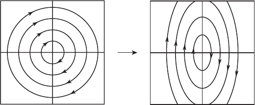
T
Figure 3.8 The change of variables T in the case of a
center.
Now, let T be the matrix whose columns are the real and imaginary parts of
the eigenvector (1, 2i). That is
T =
10
02
.
Then, we compute easily that
T
−1
AT =
02
−20
,
which is in canonical form. The phase portraits of these systems are shown
in Figure 3.8. Note that T maps the circular solutions of the system Y
=
(T
−1
AT )Y to elliptic solutions of X
= AX .
Example. (Repeated Eigenvalues) Suppose A has a single real eigen-
value λ. If there exist a pair of linearly independent eigenvectors, then in
fact A must be in the form
A =
λ 0
0 λ
,
so the system X
= AX is easily solved (see Exercise 15).
For the more complicated case, let’s assume that V is an eigenvector and
that every other eigenvector is a multiple of V . Let W be any vector for which
V and W are linearly independent. Then we have
AW = μV + νW

Exercises 57
for some constants μ, ν ∈ R. Note that μ = 0, for otherwise we would have a
second linearly independent eigenvector W with eigenvalue ν. We claim that
ν = λ.Ifν − λ = 0, a computation shows that
A
W +
μ
ν − λ
V
= ν
W +
μ
ν − λ
V
.
This says that ν is a second eigenvalue different from λ. Hence we must have
ν = λ.
Finally, let U = (1/μ)W . Then
AU = V +
λ
μ
W = V + λU .
Thus if we define TE
1
= V , TE
2
= U ,weget
T
−1
AT =
λ 1
0 λ
as required. Thus X
= AX is again in canonical form after this change of
coordinates.
EXERCISES
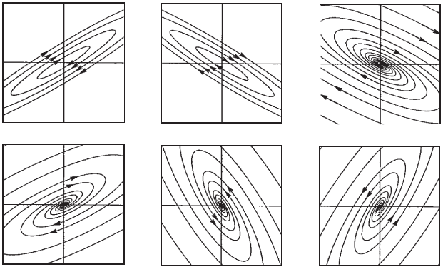
1. In Figure 3.9 on page 58, you see six phase portraits. Match each of these
phase portraits with one of the following linear systems:
(a)
35
−2 −2
(b)
−3 −2
52
(c)
3 −2
5 −2
(d)
−35
−23
(e)
35
−2 −3
(f )
−35
−22

58 Chapter 3 Phase Portraits for Planar Systems
1.
4.
2.
5.
3.
7.
Figure 3.9 Match these phase portraits with the systems in Exercise 1.
2. For each of the following systems of the form X
= AX
(a) Find the eigenvalues and eigenvectors of A.
(b) Find the matrix T that puts A in canonical form.
(c) Find the general solution of both X
= AX and Y
= (T
−1
AT )Y .
(d) Sketch the phase portraits of both systems.
(i) A =
01
10
(ii) A =
11
10
(iii) A =
11
−10
(iv) A =
11
−13
(v) A =
11
−1 −3
(vi) A =
11
1 −1
3. Find the general solution of the following harmonic oscillator equations:
(a) x
+ x
+ x = 0
(b) x
+ 2x
+ x = 0
4. Consider the harmonic oscillator system
X
=
01
−k −b
X
where b ≥ 0, k>0 and the mass m = 1.
Exercises 59
(a) For which values of k, b does this system have complex eigenvalues?
Repeated eigenvalues? Real and distinct eigenvalues?
(b) Find the general solution of this system in each case.
(c) Describe the motion of the mass when the mass is released from
the initial position x = 1 with zero velocity in each of the cases in
part (a).
5. Sketch the phase portrait of X
= AX where
A =
a 1
2a 2
.
For which values of a do you find a bifurcation? Describe the phase
portrait for a-values above and below the bifurcation point.
6. Consider the system
X
=
2ab
b 0
X.
Sketch the regions in the ab–plane where this system has different types
of canonical forms.
7. Consider the system
X
=
λ 1
0 λ
X
with λ = 0. Show that all solutions tend to (respectively, away from)
the origin tangentially to the eigenvector (1, 0) when λ < 0 (respectively,
λ > 0).
8. Find all 2 × 2 matrices that have pure imaginary eigenvalues. That is,
determine conditions on the entries of a matrix that guarantee that the
matrix has pure imaginary eigenvalues.
9. Determine a computable condition that guarantees that, if a matrix A
has complex eigenvalues, then solutions of X
= AX travel around the
origin in the counterclockwise direction.
10. Consider the system
X
=
ab
cd
X
where a + d = 0 but ad − bc = 0. Find the general solution of this
system and sketch the phase portrait.
60 Chapter 3 Phase Portraits for Planar Systems
11. Find the general solution and describe completely the phase portrait for
X
=
01
00
X.
12. Prove that
αe
λt
1
0
+ βe
λt
t
1
is the general solution of
X
=
λ 1
0 λ
X.
13. Prove that a 2×2 matrix A always satisfies its own characteristic equation.
That is, if λ
2
+αλ +β = 0 is the characteristic equation associated to A,
then the matrix A
2
+ αA + βI is the 0 matrix.
14. Suppose the 2 × 2 matrix A has repeated eigenvalues λ. Let V ∈
R
2
.
Using the previous problem, show that either V is an eigenvector for A
or else (A − λI)V is an eigenvector for A.
15. Suppose the matrix A has repeated real eigenvalues λ and there exists a
pair of linearly independent eigenvectors associated to A. Prove that
A =
λ 0
0 λ
.
16. Consider the (nonlinear) system
x
=|y|
y
=−x.
Use the methods of this chapter to describe the phase portrait.

4
Classification of
Planar Systems
In this chapter, we summarize what we have accomplished so far using a
dynamical systems point of view. Among other things, this means that we
would like to have a complete “dictionary” of all possible behaviors of 2 × 2
autonomous linear systems. One of the dictionaries we present here is geo-
metric: the trace-determinant plane. The other dictionary is more dynamic:
this involves the notion of conjugate systems.
4.1 The Trace-Determinant Plane
For a matrix
A =
ab
cd
we know that the eigenvalues are the roots of the characteristic equation, which
can be written
λ
2
− (a + d)λ + (ad − bc) = 0.
The constant term in this equation is det A. The coefficient of λ also has a
name: The quantity a + d is called the trace of A and is denoted by tr A.
61

62 Chapter 4 Classification of Planar Systems
Thus the eigenvalues satisfy
λ
2
− (tr A)λ + det A = 0
and are given by
λ
±
=
1
2
tr A ±
(tr A)
2
− 4 det A
.
Note that λ
+
+ λ
−
= tr A and λ
+
λ
−
= det A, so the trace is the sum of the
eigenvalues of A while the determinant is the product of the eigenvalues of
A. We will also write T = tr A and D = det A. Knowing T and D tells us
the eigenvalues of A and therefore virtually everything about the geometry of
solutions of X
= AX. For example, the values of T and D tell us whether
solutions spiral into or away from the origin, whether we have a center, and
so forth.
We may display this classification visually by painting a picture in the trace-
determinant plane. In this picture a matrix with trace T and determinant D
corresponds to the point with coordinates (T, D). The location of this point
in the TD–plane then determines the geometry of the phase portrait as above.
For example, the sign of T
2
− 4D tells us that the eigenvalues are:
1. Complex with nonzero imaginary part if T
2
− 4D<0;
2. Real and distinct if T
2
− 4D>0;
3. Real and repeated if T
2
− 4D = 0.
Thus the location of (T , D) relative to the parabola T
2
− 4D = 0intheTD–
plane tells us all we need to know about the eigenvalues of A from an algebraic
point of view.
In terms of phase portraits, however, we can say more. If T
2
−4D<0, then
the real part of the eigenvalues is T /2, and so we have a
1. Spiral sink if T<0;
2. Spiral source if T>0;
3. Center if T = 0.
If T
2
−4D>0 we have a similar breakdown into cases. In this region, both
eigenvalues are real. If D<0, then we have a saddle. This follows since D is the
product of the eigenvalues, one of which must be positive, the other negative.
Equivalently, if D<0, we compute
T
2
<T
2
− 4D
so that
±T<
T
2
− 4D.

4.1 The Trace-Determinant Plane 63
Thus we have
T +
T
2
− 4D>0
T −
T
2
− 4D<0
so the eigenvalues are real and have different signs. If D>0 and T<0 then
both
T ±
T
2
− 4D<0,
so we have a (real) sink. Similarly, T>0 and D>0 leads to a (real) source.
When D = 0 and T = 0, we have one zero eigenvalue, while both
eigenvalues vanish if D = T = 0.
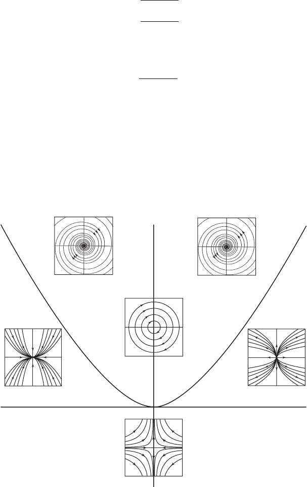
Plotting all of this verbal information in the TD–plane gives us a visual
summary of all of the different types of linear systems. The equations above
partition the TD–plane into various regions in which systems of a particular
type reside. See Figure 4.1. This yields a geometric classification of 2 ×2 linear
systems.
Det
Tr
T
2
⫽4D
Figure 4.1 The trace-determinant plane. Any resemblance to any of the
authors’ faces is purely coincidental.

64 Chapter 4 Classification of Planar Systems
A couple of remarks are in order. First, the trace-determinant plane is a
two-dimensional representation of what is really a four-dimensional space,
since 2 × 2 matrices are determined by four parameters, the entries of the
matrix. Thus there are infinitely many different matrices corresponding to each
point in the TD–plane. While all of these matrices share the same eigenvalue
configuration, there may be subtle differences in the phase portraits, such as the
direction of rotation for centers and spiral sinks and sources, or the possibility
of one or two independent eigenvectors in the repeated eigenvalue case.
We also think of the trace-determinant plane as the analog of the bifurcation
diagram for planar linear systems. A one-parameter family of linear systems
corresponds to a curve in the TD–plane. When this curve crosses the T -axis,
the positive D-axis, or the parabola T
2
− 4D = 0, the phase portrait of the
linear system undergoes a bifurcation: A major change occurs in the geometry
of the phase portrait.
Finally, note that we may obtain quite a bit of information about the system
from D and T without ever computing the eigenvalues. For example, if D<0,
we know that we have a saddle at the origin. Similarly, if both D and T are
positive, then we have a source at the origin.
4.2 Dynamical Classification
In this section we give a different, more dynamical classification of planar linear
systems. From a dynamical systems point of view, we are usually interested
primarily in the long-term behavior of solutions of differential equations.
Thus two systems are equivalent if their solutions share the same fate. To
make this precise we recall some terminology introduced in Section 1.5 of
Chapter 1.
To emphasize the dependence of solutions on both time and the initial con-
ditions X
0
, we let φ
t
(X
0
) denote the solution that satisfies the initial condition
X
0
. That is, φ
0
(X
0
) = X
0
. The function φ(t , X
0
) = φ
t
(X
0
) is called the flow of
the differential equation, whereas φ
t
is called the time t map of the flow.
For example, let
X
=
20
03
X.
Then the time t map is given by
φ
t
(x
0
, y
0
) =
x
0
e
2t
, y
0
e
3t
.
Thus the flow is a function that depends on both time and the initial values.

4.2 Dynamical Classification 65
We will consider two systems to be dynamically equivalent if there is a
function h that takes one flow to the other. We require that this function be
a homeomorphism, that is, h is a one-to-one, onto, and continuous function
whose inverse is also continuous.
Definition
Suppose X
= AX and X
= BX have flows φ
A
and φ
B
. These two
systems are (topologically) conjugate if there exists a homeo-
morphism h :
R
2
→ R
2
that satisfies
φ
B
(t, h(X
0
)) = h(φ
A
(t, X
0
)).
The homeomorphism h is called a conjugacy. Thus a conjugacy
takes the solution curves of X
= AX to those of X
= BX .
Example. For the one-dimensional linear differential equations
x
= λ
1
x and x
= λ
2
x
we have the flows
φ
j
(t, x
0
) = x
0
e
λ
j
t
for j = 1, 2. Suppose that λ
1
and λ
2
are nonzero and have the same sign.
Then let
h(x) =
⎧
⎪
⎨
⎪
⎩
x
λ
2
/λ
1
if x ≥ 0
−|x|
λ
2
/λ
1
if x<0
where we recall that
x
λ
2
/λ
1
= exp
λ
2
λ
1
log(x)
.
Note that h is a homeomorphism of the real line. We claim that h is a conjugacy
between x
= λ
1
x and x
= λ
2
x. To see this, we check that when x
0
> 0
h(φ
1
(t, x
0
)) =
x
0
e
λ
1
t
λ
2
/λ
1
