Hirsch M., Smale S., Devaney R., Differential Equations, Dynamical Systems, and an Introduction to Chaos

Подождите немного. Документ загружается.

106 Chapter 5 Higher Dimensional Linear Algebra

Prove that S may be written as the collection of all possible linear

combinations of a ﬁnite set of vectors.

13. Which of the following subsets of

are open and/or dense? Give a brief

reason in each case.

(a)

={(x, y) |y>0};

(b)

={(x, y) |x

+ y

= 1};

(c)

={(x, y) |x is irrational};

(d)

={(x, y) |x and y are not integers};

(e)

is the complement of a set C

where C

is closed and not dense;

(f)

is the complement of a set C

which contains exactly 6 billion and

two distinct points.

14. Each of the following properties deﬁnes a subset of real n × n matrices.

Which of these sets are open and/or dense in the L(

)? Give a brief

reason in each case.

(a) det A = 0.

(b) Trace A is rational.

(d) 3 ≤ det A<4.

(e) −1 < |λ| < 1 for every eigenvalue λ.

(f) A has no real eigenvalues.

(g) Each real eigenvalue of A has multiplicity one.

15. Which of the following properties of linear maps on

are generic?

(a) |λ| = 1 for every eigenvalue λ.

(b) n = 2; some eigenvalue is not real.

(d) No solution of X



= AX is periodic (except the zero solution).

(e) There are n distinct eigenvalues, each with distinct imaginary parts.

(f) AX = X and AX =−X for all X = 0.

Higher Dimensional

Linear Systems

After our little sojourn into the world of linear algebra, it’s time to return to dif-

ferential equations and, in particular, to the task of solving higher dimensional

linear systems with constant coefﬁcients. As in the linear algebra chapter, we

have to deal with a number of different cases.

6.1 Distinct Eigenvalues

Consider ﬁrst a linear system X



= AX where the n × n matrix A has n

distinct, real eigenvalues λ

, ..., λ

. By the results in Chapter 5, there is a

change of coordinates T so that the new system Y



= (T

−1

AT )Y assumes the

particularly simple form



= λ



= λ

The linear map T is the map that takes the standard basis vector E

to the

eigenvector V

associated to λ

. Clearly, a function of the form

Y (t ) =

⎛

⎜

⎝

⎞

⎟

⎠

107

108 Chapter 6 Higher Dimensional Linear Systems

is a solution of Y



= (T

−1

AT )Y that satisﬁes the initial condition Y (0) =

, ..., c

). As in Chapter 3, this is the only such solution, because if

W (t) =

⎛

⎜

⎝

(t)

⎞

⎟

⎠

is another solution, then differentiating each expression w

(t) exp(−λ

t), we

ﬁnd

(t)e

−λ

= (w



− λ

−λ

= 0.

Hence w

(t) = c

exp(λ

t) for each j. Therefore the collection of solutions

Y (t ) yields the general solution of Y



= (T

−1

AT )Y .

It then follows that X (t ) = TY (t) is the general solution of X



= AX,so

this general solution may be written in the form

X(t ) =



j=1

Now suppose that the eigenvalues λ

, ..., λ

of A are negative, while the

eigenvalues λ

k+1

, ..., λ

are positive. Since there are no zero eigenvalues, the

system is hyperbolic. Then any solution that starts in the subspace spanned

by the vectors V

, ..., V

must ﬁrst of all stay in that subspace for all time

since c

k+1

=···=c

= 0. Secondly, each such solution tends to the origin

as t →∞. In analogy with the terminology introduced for planar systems,

we call this subspace the stable subspace. Similarly, the subspace spanned by

k+1

, ..., V

contains solutions that move away from the origin. This subspace

is the unstable subspace. All other solutions tend toward the stable subspace

as time goes backward and toward the unstable subspace as time increases.

Therefore this system is a higher dimensional analog of a saddle.

Example. Consider



⎛

⎝

12−1

03−2

02−2

⎞

⎠

In Section 5.2 in Chapter 5, we showed that this matrix has eigenvalues

2, 1, and −1 with associated eigenvectors (3, 2, 1), (1, 0, 0), and (0, 1, 2),

respectively. Therefore the matrix

T =

⎛

⎝

310

201

102

⎞

⎠

6.1 Distinct Eigenvalues 109

(0, 1, 2)

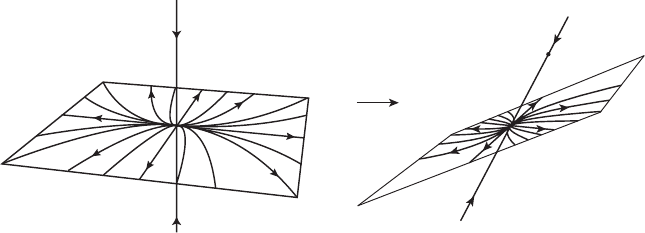
Figure 6.1 The stable and unstable subspaces of a saddle in dimension 3.

On the left, the system is in canonical form.

converts X



= AX to



= (T

−1

AT )Y =

⎛

⎝

20 0

01 0

00−1

⎞

⎠

Y ,

which we can solve immediately. Multiplying the solution by T then yields the

general solution

X(t ) = c

⎛

⎝

⎞

⎠

+ c

⎛

⎝

⎞

⎠

+ c

−t

⎛

⎝

⎞

⎠

of X



= AX. The straight line through the origin and (0, 1, 2) is the stable

line, while the plane spanned by (3, 2, 1) and (1, 0, 0) is the unstable plane. A

collection of solutions of this system as well as the system Y



= (T

−1

AT )Y is

displayed in Figure 6.1.



Example. If the 3 × 3 matrix A has three real, distinct eigenvalues that are

negative, then we may ﬁnd a change of coordinates so that the system assumes

the form



= (T

−1

AT )Y =

⎛

⎝

0 λ

00λ

⎞

⎠

where λ

< λ

< 0. All solutions therefore tend to the origin and so

we have a higher dimensional sink. See Figure 6.2. For an initial condition

, y

, z

) with all three coordinates nonzero, the corresponding solution

tends to the origin tangentially to the x-axis (see Exercise 2 at the end of

the chapter).



110 Chapter 6 Higher Dimensional Linear Systems

Figure 6.2 A sink in three dimensions.

Now suppose that the n × n matrix A has n distinct eigenvalues, of which

are real and 2k

are nonreal, so that n = k

+ 2k

. Then, as in Chapter 5,

we may change coordinates so that the system assumes the form



= λ





= α



+ β







=−β



+ α



for j = 1, ..., k

and  = 1, ..., k

. As in Chapter 3, we therefore have solutions

of the form

(t) = c



(t) = p



cos β



t + q



sin β



(t) =−p



sin β



t + q



cos β



As before, it is straightforward to check that this is the general solution. We

have therefore shown:

Theorem. Consider the system X



= AX where A has distinct eigenvalues

, ..., λ

∈ R and α

+iβ

, ..., α

+iβ

∈ C. Let T be the matrix that puts

A in the canonical form

−1

AT =

⎛

⎜

⎝

⎞

⎟

⎠

6.1 Distinct Eigenvalues

111

where



−β



Then the general solution of X



= AX is TY (t ) where

Y (t ) =

⎛

⎜

⎝

cos β

t + b

sin β

−a

sin β

t + b

cos β

t + b

sin β

−a

sin β

t + b

cos β

⎞

⎟

⎠



As usual, the columns of the matrix T in this theorem are the eigenvectors

(or the real and imaginary parts of the eigenvectors) corresponding to each

eigenvalue. Also, as before, the subspace spanned by the eigenvectors corre-

sponding to eigenvalues with negative (resp., positive) real parts is the stable

(resp., unstable) subspace.

Example. Consider the system



⎛

⎝

010

−100

00−1

⎞

⎠

whose matrix is already in canonical form. The eigenvalues are ±i, −1. The

solution satisfying the initial condition (x

, y

, z

) is given by

Y (t ) = x

⎛

⎝

cos t

−sin t

⎞

⎠

+ y

⎛

⎝

sin t

cos t

⎞

⎠

+ z

−t

⎛

⎝

⎞

⎠

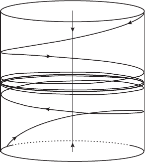
so this is the general solution. The phase portrait for this system is displayed

in Figure 6.3. The stable line lies along the z-axis, whereas all solutions in the

xy–plane travel around circles centered at the origin. In fact, each solution

that does not lie on the stable line actually lies on a cylinder in

given by

+ y

= constant. These solutions spiral toward the circular solution of

radius



+ y

in the xy–plane if z

= 0. 

112 Chapter 6 Higher Dimensional Linear Systems

⫹y

⫽a

Figure 6.3 The phase portrait for a spiral

center.

Example. Now consider X



= AX where

A =

⎛

⎝

−0. 1 0 1

−11−1. 1

−10−0. 1

⎞

⎠

The characteristic equation is

−λ

+ 0. 8λ

− 0. 81λ + 1. 01 = 0,

which we have kindly factored for you into

(1 − λ)(λ

+ 0. 2λ + 1. 01) = 0.

Therefore the eigenvalues are the roots of this equation, which are 1 and −0. 1±

i. Solving (A −(−0. 1 + i)I )X = 0 yields the eigenvector (−i, 1, 1) associated

to −0. 1 + i. Let V

= Re (−i,1,1) = (0, 1, 1) and V

= Im (−i,1,1) =

(−1, 0, 0). Solving (A − I)X = 0 yields V

= (0, 1, 0) as an eigenvector

corresponding to λ = 1. Then the matrix whose columns are the V

T =

⎛

⎝

0 −10

101

100

⎞

⎠

6.1 Distinct Eigenvalues 113

Figure 6.4 A spiral saddle in canonical

form.

converts X



= AX into



⎛

⎝

−0.110

−1 −0. 1 0

001

⎞

⎠

Y .

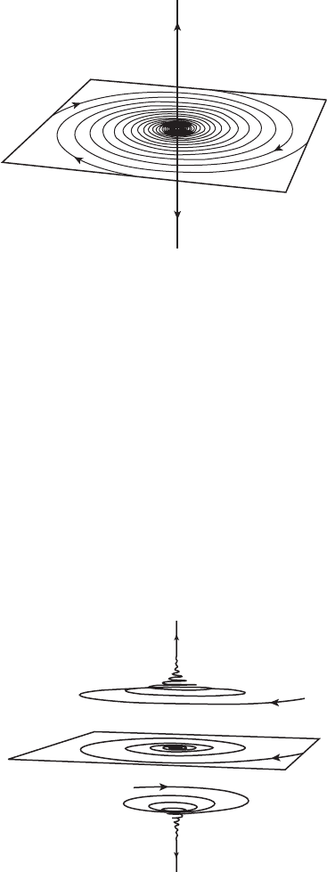
This system has an unstable line along the z-axis, while the xy–plane is the

stable plane. Note that solutions spiral into 0 in the stable plane. We call

this system a spiral saddle (see Figure 6.4). Typical solutions of the stable

plane spiral toward the z-axis while the z-coordinate meanwhile increases or

decreases (see Figure 6.5).



Figure 6.5 Typical solutions of the spiral

saddle tend to spiral toward the unstable

line.

114 Chapter 6 Higher Dimensional Linear Systems

6.2 Harmonic Oscillators

Consider a pair of undamped harmonic oscillators whose equations are



=−ω



=−ω

We can almost solve these equations by inspection as visions of sin ωt and

cos ωt pass through our minds. But let’s push on a bit, ﬁrst to illustrate the

theorem in the previous section in the case of nonreal eigenvalues, but more

importantly to introduce some interesting geometry.

We ﬁrst introduce the new variables y

= x



for j = 1, 2 so that the equations

can be written as a system



= y



=−ω

In matrix form, this system is X



= AX where X = (x

, y

, x

, y

) and

A =

⎛

⎜

⎝

−ω

⎞

⎟

⎠

This system has eigenvalues ±iω

and ±iω

. An eigenvector corresponding to

iω

is V

= (1, iω

, 0, 0) while V

= (0, 0, 1, iω

) is associated to iω

. Let W

and W

be the real and imaginary parts of V

, and let W

and W

be the same

for V

. Then, as usual, we let TE

= W

and the linear map T puts this system

into canonical form with the matrix

−1

AT =

⎛

⎜

⎝

0 ω

−ω

0 ω

−ω

⎞

⎟

⎠

We then derive the general solution

Y (t ) =

⎛

⎜

⎝

(t)

⎞

⎟

⎠

⎛

⎜

⎝

cos ω

t + b

sin ω

−a

sin ω

t + b

cos ω

t + b

sin ω

−a

sin ω

t + b

cos ω

⎞

⎟

⎠

just as we originally expected.

6.2 Harmonic Oscillators 115

We could say that this is the end of the story and stop here since we have the

formulas for the solution. However, let’s push on a bit more.

Each pair of solutions (x

(t), y

(t)) for j = 1, 2 is clearly a periodic solution

of the equation with period 2π/ω

, but this does not mean that the full four-

dimensional solution is a periodic function. Indeed, the full solution is a peri-

odic function with period τ if and only if there exist integers m and n such that

τ = m · 2π and ω

τ = n · 2π .

Thus, for periodicity, we must have

τ =

2πm

2πn

or, equivalently,

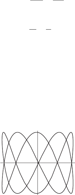
That is, the ratio of the two frequencies of the oscillators must be a rational

number. In Figure 6.6 we have plotted (x

(t), x

(t)) for particular solution of

this system when the ratio of the frequencies is 5/2.

When the ratio of the frequencies is irrational, something very different

happens. To understand this, we make another (and much more familiar)

change of coordinates. In canonical form, our system currently is



= ω



=−ω

Figure 6.6 A solution with

frequency ratio 5/2 projected

into the x

–plane. Note that

(t) oscillates five times and

(t) only twice before returning

to the initial position.