Hillert M. Phase Equilibria, Phase Diagrams and Phase Transformations: Their Thermodynamic Basis

Подождите немного. Документ загружается.

17.6 Mechanisms of interface migration 395

α/β

β/α

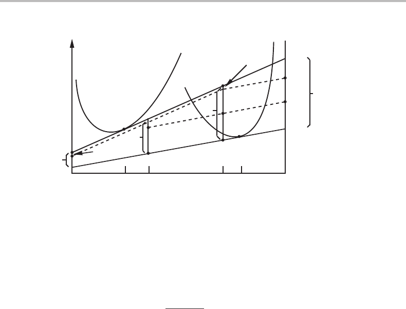
Figure 17.3 Precipitation of β from α by three processes, individual diffusion of A and B and a

cooperative mechanism. The dissipations per mole of transferred atoms are obtained from each

driving force multiplied by the fraction of its ﬂux, f

= J

/(J

+  J

An alternative way of reducing the net effect of the three processes to an effect of

two may be preferable. One would then divide the cooperative ﬂux on the individual

components obtaining J

= x

.For the total ﬂux of component j one would then

obtain

total

= J

+ x

α/β

β/α

(−µ

) + x

α:β

)



(−µ

)

(17.68)

Then one could determine the composition of the cooperative mechanism by inserting

Eq. (17.68) into Eq. (17.56), whose right-hand side is given by the ﬂuxes inside the α

and β phases.

We can now see from Eq. (17.68) that by adding the cooperative mechanism to the

individual diffusion of the components we have actually entered cross terms into the

individual phenomenological equations. It may thus seem that one could have obtained

the same effect by taking cross terms into account directly without modelling any mech-

anism. However, there is a major difference. Through the presence of x

and x

Eq. (17.68), which are related to the ﬂuxes inside the phases through Eq. (17.56), it

is possible to make the cross coefﬁcients change automatically as the growth conditions

vary during a process. Furthermore, through Eq. (17.68) the cross coefﬁcients of various

components are related and the summation in Eq. (17.68) also contains a term for the

component under consideration, i.e. for i = j,and it will also change with the growth con-

ditions. Finally, it will also be easy to introduce a non-linear kinetic law for the cooperative

part of the phase transformation by making the mobility M

α:β

depend on the velocity.

Exercise 17.8

Prove that the introduction of the processes deﬁned by Eqs (17.60) to (17.63) actually

kept the rate of entropy production invariant.

396 Kinetics of transport processes

Hint

One can add



− x





(

− D

)

which is equal to zero.

Solution



i=1

∗

n−1



i=1



− x





(

− D

)



i=1



i=1



− J

− x



k=1

+ x



k=1





k=1



i=1



i=1

− D



i=1

−



k=1



i=1

+ D



k=1



i=1



k=1



i=1



i=1

17.7 Balance of forces and dissipation

We shall now examine how the driving forces and dissipations of Gibbs energy are

balanced in a simple case of diffusional phase transformation. The equation for diffusion

by the vacancy mechanism will be applied. A limited mobility of the interfaces will also

be considered. Svoboda et al.[36] has emphasized that this is a case where it may be an

advantage to apply Onsager’s extremum principle from Section 5.9 because one cannot

make any a priori assumption about the conditions at the migrating interfaces if there

is friction in them and those conditions are usually required as boundary conditions for

solving the diffusion equations inside the phases. We shall follow that procedure.

We shall consider a binary case where all phases have almost constant compositions

and a β phase is being formed from an initial interface between an A-rich α phase and

a B-rich γ phase. In α and γ there will be no diffusion. The system is shaped as a rod

with a constant cross-section of a and with the α:γ interface perpendicular to the length

coordinate. Because the β phase has an almost constant composition, the ﬂuxes of A or

B can at each moment be approximated as constant through the whole length of β.

First we must ﬁnd the rate of change of Gibbs energy of the whole system. Gibbs

energy per area a of the rod is

G/a = l



, (17.69)

wherel

is the length of the respective phase. The velocities of the interfaces are obtained

from the time derivatives of l

and the rate of change of Gibbs energy will be



= G

α/β

− G

β/α

+ G

β/γ

− G

γ/β

. (17.70)

17.7 Balance of forces and dissipation 397

∆µ

α/β

β/γ

α/β

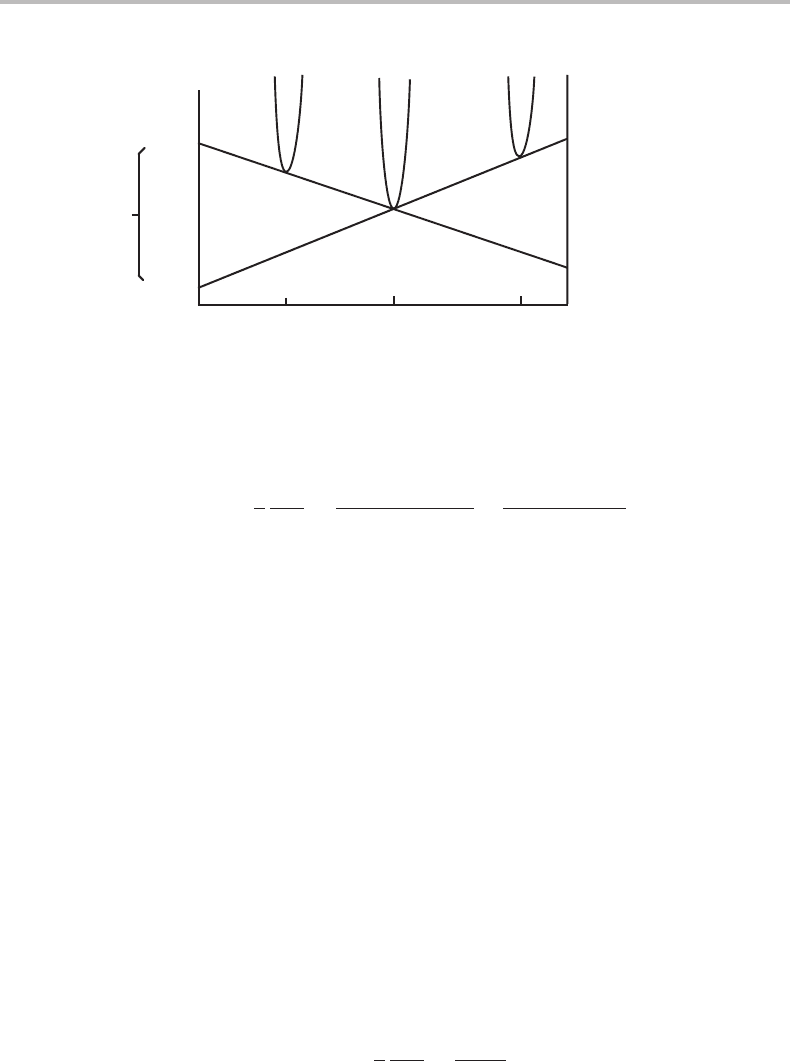
Figure 17.4 Molar Gibbs energy diagram for a system with three phases. A will diffuse from the

α/β interface to the β/γ interface and B in the other direction. β will grow into both α and γ.

By inserting the velocities from Eqs (17.49) and (17.50)wecan evaluate two driving

forces for diffusion through the β phase, ∂

G/∂ J

and ∂

G/∂ J

∂

∂ J

−G

+ G

− x

− G

− x

. (17.71)

Figure 17.4 illustrates that this result can be expressed as µ

= µ

β/γ

− µ

α/β

,where

the chemical potentials are evaluated for full equilibrium between the phases across the

interface, as if there were no losses in the interface. The diagram shows that µ

negative and we have thus a positive driving force for diffusion of A in the direction

from α to γ.Onthe other hand, µ

will be positive and the driving force for B would

thus drive B in the opposite direction.

The rate of dissipation of Gibbs energy for a process is given by Eq. (5.133)ifthe

cross coefﬁcients can be neglected,

= X

= (1/L

. (17.72)

We shall ﬁrst apply this to the two individual diffusion processes. As explained below

Eq. (17.6), for diffusion this is the dissipation per volume of the phase. We can easily

integrate over the whole length of the β phase because the ﬂuxes can be treated as

constant, as already explained. The volume of the β phase is a · l

and the diffusion

equation, Eq. (17.10), yields for diffusion of A,

= al



= al



. (17.73)

We shall soon need the derivative with respect to the diffusion ﬂuxes, e.g.,

∂φ

∂ J

. (17.74)

The present problem would have been trivial if the two diffusion processes were the

only ones to consider. However, we shall also consider friction of the migrating interface

caused by a cooperative mechanism. For that process one would perhaps like to apply

Eq. (17.4)but there is a problem because, according to Section 17.5, there are two

398 Kinetics of transport processes

different velocities depending on what lattice is used as reference. The difference is

caused by the two elements having different diffusivities in the β phase. The velocity

relative to the lattice of the β phase is affected by the difference resulting in a net

transportation of vacancies to or from the interface. However, there is no diffusion in

the α phase and the velocity relative to that lattice is caused only by the atoms crossing

the interface. We shall thus use υ

α/β

from Eq. (17.49). Furthermore, there is a factor

on the right-hand side of Eq. (17.4)which may also be different for the two phases.

However, it was eliminated in Eq. (17.5) although the choice of V

in Eq. (17.4) has

affected the value of the mobility M. The rate of dissipation of Gibbs energy due to the

friction in the interface is thus obtained as

T σ

α/β

= φ

α/β

= aυ

α/β



−G





= a

α/β

(υ

α/β

)

= a





α/β



α/β



(17.75)

Comparison with Eq. (17.73) shows that the thickness of the interface has been included

in the mobility. Using Eq. (17.49)wecan evaluate the derivatives with respect to the

ﬂuxes,

∂φ

α/β

∂ J





α/β

−x

− x

. (17.76)

We get similar equations for the β/γ interface. The complete dissipation function will

 = φ

+ φ

α/β

+ φ

β/γ

. (17.77)

We can evaluate ∂/∂J

and ∂/∂J

and Onsager’s extremum principle, Eq. (5.141),

yields two kinetic equations,

−

∂

∂ J

∂

∂ J

, (17.78)

where i is either A or B. In principle we can thus solve for J

and J

.Wecan insert

the right-hand side of Eq. (17.71), which is equal to µ

according to Fig. 17.4, and of

Eq. (17.74). By ﬁrst omitting the effects of the friction in the interfaces we ﬁnd

− µ

; − µ

(17.79)

(−µ

); J

=−

µ

. (17.80)

These are well-known equations obtainable by classical methods. However, the result

will be more complicated byincluding the effectsfrom the interfaces givenbyEq. (17.76).

− µ





α/β

−x

− x





β/γ

γ/β

− x

. (17.81)



−µ





α/β

− x

−





β/γ

γ/β

− x



. (17.82)

17.7 Balance of forces and dissipation 399

In the present case where β grows into both α and γ, υ

α/β

is negative and υ

γ/β

positive. Equation (17.82) demonstrates that for weak effects of friction they may both

be regarded as negative corrections to the driving force, −µ

, caused by deviations

from local equilibrium at the interfaces. For stronger effects it may be more natural to

regard them as dissipations of Gibbs energy as in Eq. (17.81). There may be a numerical

problem because the contributions from the interfaces contain the velocities and they are

functions of the ﬂuxes. However, with computerized methods there should be no great

problem.

With this example we have demonstrated that even in a case with several processes

that dissipate Gibbs energy it may be possible to formulate the kinetic equations directly.

Methods of modelling

18.1 General principles

By ‘modelling’ we shall understand the selection of some assumptions from which it is

possible to calculate the properties of a system. Sometimes it is possible to obtain a close

mathematical expression giving a property as a function of interesting variables. In this

chapter and the following ones we shall mainly concern ourselves with such models.

However, in many cases the model cannot be expressed in a closed mathematical form

but results can also be obtained by numerical calculations using some iterative method.

When the iteration in some way resembles the behaviour of a real physical system one

talks about ‘simulation’. Such methods are becoming increasingly more powerful thanks

to access to more and more powerful computers.

The purpose of modelling is two-fold. From a scientiﬁc point of view one likes to

learn how nature functions. One way of gaining knowledge is to deﬁne some hypothesis

resulting in a model and test it by comparing the predictions from the model with

experimental information. Then, it does not matter much if the predictions are made

by an analytical calculation or by some numerical method. From a more technological

point of view one likes to predict the properties of a particular system in order to put it to

efﬁcient use in some practical construction or operation. Then it is often most convenient

to have a model which yields an analytical expression.

In the simplest case, modelling is just the selection of a mathematical form which has

proved useful, whether it is based on some physical model or not. However, experience

shows that a model is usually more powerful if it is based upon physically sound princi-

ples. With such a model one can hope to make predictions outside the tested range with

some conﬁdence.

The ﬁrst question to discuss is what thermodynamic function to model. That question

will be addressed in the next section.

Exercise 18.1

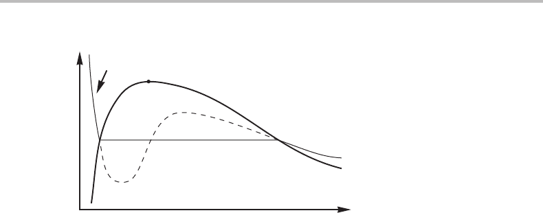
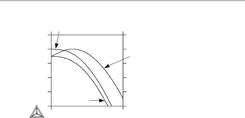
Figure 18.1 shows a P, V diagram for a pure substance at a high temperature where only

gas and liquid exist. Above the critical point c there is no sharp difference between the

two phases. It is thus tempting to try to apply a single mathematical model for both phases

but it would then give values also for one-phase states inside the two-phase ﬁeld, i.e.,

below the thick line. Such states would be metastable or unstable. The thermodynamic

18.2 Choice of characteristic state function 401

gas

isotherm

Figure 18.1 See Exercise 18.1.

properties of unstable states may be questioned but it seems reasonable at least to obey

basic thermodynamic principles when constructing the model.

The thin line represents an isotherm. Show that the model must be constructed in such

away that the two areas A

and A

are equal. Actually, this is a way of identifying the

equilibrium points, L

and gas

,onthe curve from a model that extends over the whole

range (sometimes called Maxwell’s construction).

Hint

Evaluate the change in Gibbs energy along the dashed line. It is an isothermal change and

thus dG = V dP − SdT = V dP. Then remember that the Gibbs energy of L

and gas

must be equal because they represent two states of the same substance in equilibrium

with each other at given values of P and T.

Solution

G(gas

) − G(L

) =



V dP = A

− A

. But G(gas

) = G(L

). Thus, A

= A

. This

result demonstrates that satisfactory modelling is more than just choosing a mathematical

expression.

18.2 Choice of characteristic state function

From a practical point of view we are most interested in models giving the Gibbs energy

which has temperature and pressure as its natural variables. They are usually the most

convenient experimental variables. On the other hand, the physical model itself may

make a different choice more natural. An example is the effect of thermal vibrations of

the atoms. The frequencies depend upon the forces between atoms which in turn, depend

upon the atomic distances. In that case it is most straightforward to consider the effect

under a constant volume in spite of the fact that the vibrations themselves tend to expand

the system. It is thus natural to consider the Helmholtz energy. The formation of thermal

vacancies is a very different case. There the physical picture is that an atom is removed

402 Methods of modelling

from the interior of a crystal and placed on the surface. The volume is thus increased by

one lattice site. If the atomic distances are to be kept constant, it is now necessary to let

the volume increase. It will thus be more straightforward to consider this process under

a constant pressure and to work with the Gibbs energy. It may be emphasized that one

should choose to model the internal energy only for a case where it is natural to consider

entropy and volume as constant and that may be very rare. On the other hand, there may

be cases where the internal energy and the volume are kept constant and one could then

model the entropy.

A different question is how to model the simultaneous effects of two different phe-

nomena. It is true that the law of additivity applies to all the extensive state functions as

farascontributions from different parts of the system are concerned. However, it must be

remembered that the internal energy, volume or entropy of the whole system is then the

sum of the values for the parts, whereas the variables T and P are often the same in all the

parts and in the whole system. If there are curved interfaces between different parts then

the parts may be under different pressures and it must be remembered that the variable

P in the Gibbs energy for the whole system refers to the externally applied pressure. It

may then be more straightforward to consider the Helmholtz energy but, even so, one

must take into account the effect of the actual pressure inside each part because it affects

the molar volume.

The situation is quite different if each one of two phenomena applies to the whole

system. Each phenomenon may contribute to the total pressure which may be regarded

as the sum of two partial pressures but only if the two phenomena do not interact with

each other. On the other hand, the two phenomena in this case refer to the same volume.

In the present chapter the discussion of modelling will simply be limited to the use of

Gibbs energy.

Exercise 18.2

What would be the most natural quantity to use in a model of evaporation of a solid?

Hint

Consider which state variables should be kept constant in order to leave the bulk of the

solid unaffected by the process of evaporation.

Solution

It is not convenient to require that the volume should stay constant because then one

must compress the solid to make room for the vapour. The bulk will be unaffected if the

pressure is kept constant. One should thus model the Gibbs energy.

18.3 Reference states

As an introduction to our discussion of the modelling of the Gibbs energy it is instructive

to examine some real cases. The Gibbs energy is always given relative to some reference.

18.3 Reference states 403

bcc

–

fcc

hcp

–

fcc

liq

–

fcc

−10

0 2000

T (K)

(kJmol)

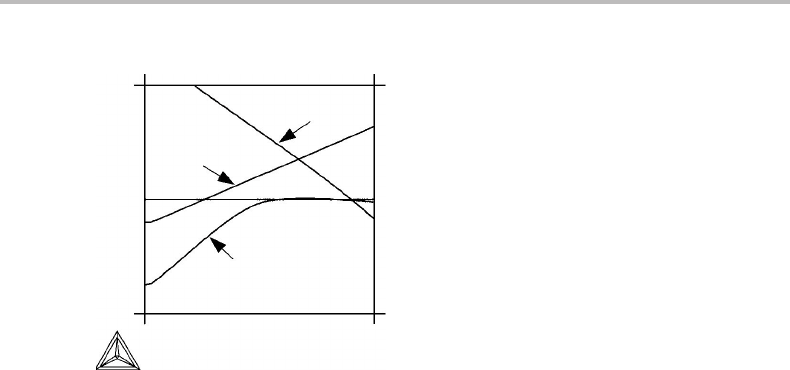
Figure 18.2 The Gibbs energy of various forms of iron, given relative to the fcc form at the same

temperature and a pressure of 1 bar.

As an example, if one inquires about the Gibbs energy for the various forms of pure solid

iron one may ﬁnd information on all the other forms relative to the fcc form. Figure 18.2

shows how these Gibbs energy differences vary with temperature at 1 bar. It is a striking

feature that such curves are often rather straight but in some regions the curvature is

strong.

Since the negative slope of these curves is identical to the entropy difference between

the two phases, we may conclude that the entropy difference is often rather constant.

In regions of strong curvature there is a strong variation of the entropy difference and

this should in turn be due to some special physical effect. The strong curvature in

bcc

−

fcc

above 1000 K is due to the magnetic transition in bcc–Fe with a Curie

temperature at 1043 K. It is evident that in order to model this curve one must include

a description of the magnetic contribution to the Gibbs energy. Furthermore, all the

curves start out parallel to the T axis at absolute zero in accordance with the third law

which states that all ordered forms of a substance should approach the same entropy

at absolute zero. On heating from absolute zero, a difference in entropy between the

various forms develops at fairly low temperatures resulting in strong curvatures. This is

due to differences in the vibration frequencies, a factor which evidently must be taken

into account in modelling these curves at low temperatures. These two physical factors

(magnetic and vibrational) will be discussed in some detail in Chapter 19. Except for

such speciﬁc physical phenomena the Gibbs energy difference is often described with

fairly simple mathematical expressions. The use of a power series in T will be described

in the next section.

Before discussing the use of a power series it is useful to examine a different way of

choosing the reference for the Gibbs energy. When representing the Gibbs energy for

a substance as a function of T, one can use as reference the same substance at some

constant T and P.Asanexample, Fig. 18.3 shows the Gibbs energy of graphite as a

function of T at 1 bar, and three different curves are presented because three different

references have been used.

It is evident that changing the choice of reference does not always displace the curve

vertically; the slope may also be affected. This is due to the fact that Gibbs energy may

404 Methods of modelling

∆G

′

= G–H(0)+TS(0)

∆G

′′

= G −H(298) +TS(298)

T (K)

(kJ/mol)

−H

SER

0 1000

−2

−4

−6

−8

Figure 18.3 The Gibbs energy of graphite, given relative to various references. The pressure is

1 bar.

be regarded as composed of an enthalpy part and an entropy part and neither of these

quantities has a natural zero point. In reality, one must deﬁne references for both. This

can be done by choosing graphite of some temperature, e.g. 0 or 298.15 K. The quantities

plotted with these choices are





(T ) −

(0) + T

(0) (18.1)





(T ) −

(298) + T

(298), (18.2)

where 298.15 K has been abbreviated as 298. The slope of the curves is obtained as

d



/dT =−

(T ) +

(0) (18.3)

d



/dT =−

(T ) +

(298). (18.4)

These are both satisfactory results.

It is also possible to deﬁne the references for H and S using different states. A rather

popular choice is the following



(T ) −

(298) + T

(0). (18.5)

It is usually combined with the convention to set

(0) to zero. The last term is thus

omitted. Furthermore,

(298) is often chosen as the value for the element in its most

stable form at 298 K and 1 bar, a quantity which is sometimes denoted by H

SER

for stable

element reference. This is why the third curve in Fig. 18.3 is identiﬁed as

− H

SER

When no reference entropy is given, it means that one has in fact chosen

(0) and set

this quantity to zero. In any case, it is not necessary to decide on the choice of reference

until one wants to put in numerical values. In the present text we shall use the notation

REF

and it mainly serves the purpose of reminding us that for each element one should

normally decide on a particular choice and then stick to it. However, it is only after one

has started to put in numbers that one must not change the reference.