Gubbins D., Herrero-Bervera E. Encyclopedia of Geomagnetism and Paleomagnetism

Подождите немного. Документ загружается.

of the BC branch tend to extend beyond the ray theoretical predictions.

For epicentral distances beyond the C point, there is the possibility of

diffraction around the inner core. At the B caustic the real branch does

not just stop and there will be frequency dependent decay into the sha-

dow side of the caustic. In addition scattering in the mantle from PKP

produces short-period arrivals as precursors to PKIKP that can be seen

because they arrive in a quiet portion of the seismic record. The envel-

ope of possible precursors is indicated in Figure S24.

The pattern of branches for the SKS phase is somewhat different

because the P wavespeed at the top of the core is higher than the S

at the base of the mantle.

The AC branch extends from S incident on the core-mantle bound-

ary that can just propagate as P at the top of the outer core and emerge

at A  63



, through to grazing incidence at the inner core boundary at

C. Diffracted waves around the inner core can extend the branch

beyond the formal C point. The DF branch (SKIKS) again corresponds

to refracted waves in the inner core. The postcritical reflections from

the inner core boundary (SKiKS) form the CD branch and connect

directly into the precritical reflection at shorter distances than the D

point at 104



(Figure S25).

When the refraction just begins at A, the S wave path to the same

epicentral distance is shorter and SKS is about 75 s behind S. However,

as the proportion of faster P wave path in the core increases, the dis-

crepancies in S and SKS travel time are reduced. Eventually, the travel

time of SKS becomes less than that for S at the same epicentral

distance. Beyond 83



SKS becomes the onset of the shear wave group

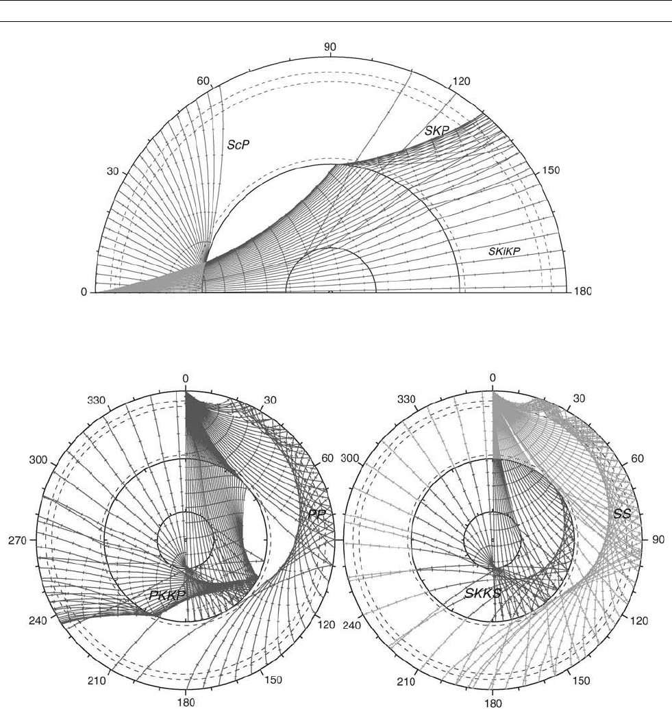
Figure S22 Ray paths for the converted phases ScP and SKiKP.

Figure S23 Ray paths for multiply reflected phases (a) PP, PKKP, (b) SS, SKKS.

906 SEISMIC PHASES

and vertically polarized S, Sdiff have to be sought in the SKS coda. The

transversely polarized S wave is very distinct and small precursory

SKS contributions (as in Figure S18) can arise from either anisotropy

of heterogeneity in passage through the mantle.

Brian Kennett

Bibliography

Duess, A., Woodhouse, J.H., Paulssen, H., and Trampert, J., 2000. The

observation of inner core shear phases. Geophysical Journal Inter-

national, 142:67–73.

Kennett, B.L.N., 2002. The Seismic Wavefield II: Interpretation

of seismograms on regional and global scales. Cambridge:

Cambridge University Press.

Kennett, B.L.N., Engdahl, E.R., and Buland, R., 1995. Constraints on

seismic velocities in the Earth from travel times. Geophysical

Journal International, 122: 108–124.

Shearer, P.M., 1999. An Introduction to Seismology. Cambridge:

Cambridge University Press.

Stein, S., and Wysession, M., 2003. An Introduction to Seismology,

Earthquakes, and Earth Structure. Oxford: Blackwell Publishing.

Cross-references

Earth Structure, Major Divisions

Inner Core, PKJKP

Inner Core Seismic Velocities

Lehmann, Inge (1888–1993)

Oldham, Richard Dixon (1858–1936)

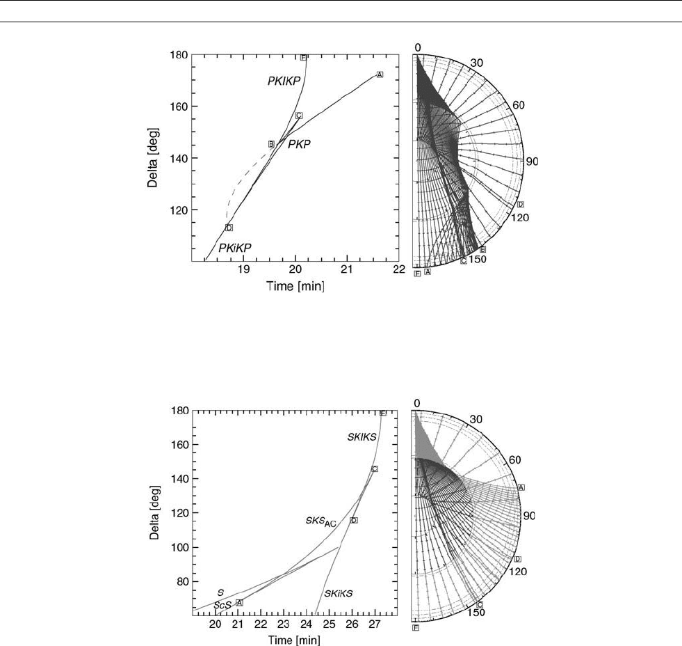
Figure S24 Rays and travel times for PKP for the AK135 model, wavefronts are indicated by tick marks at 60 s intervals. The critical

points for the various PKP branches are indicated on both the travel time curve and the ray pattern. The dashed segment indicates the

locus of precursors to PKIKP from scattering at the core-mantle boundary.

Figure S25 Rays and travel times for SKS for the AK 135 model. S legs are plotted in grey and wavefronts are indicated by tick marks at

60 s intervals. The critical points for the various SKS branches are indicated on both the travel time curves and the ray pattern.

SEISMIC PHASES 907

SEISMO-ELECTROMAGNETIC EFFECTS

Seismo-electromagnetic effects refer to electromagnetic (EM) signals

generated by fault failure processes in the Earth’s crust. These may

occur slowly (when associated with plate tectonic loading, slow earth-

quakes, postseismic slip, etc.) or rapidly preceding, during and follow-

ing earthquakes. Several different physical processes related to crustal

failure can contribute to the generation of seismo-electromagnetic

(SEM) effects. Unambiguous observations of SEM effects provide

new independent information about the physics of fault failure. Causal

relations between co-seismic magnetic field changes and earthquake

stress drops have been clearly documented. However, despite several

decades of high quality monitoring, clear demonstration of the

existence of precursory EM signals has not been achieved.

Brief history

Suggestions that electromagnetic field disturbances are a consequence

of crustal failure processes have been made throughout recorded

history. Unfortunately, much of the earliest work was recognized

as spurious by Reid (1914) who showed that transients recorded by

magnetographs located close to earthquake epicenters resulted from

earthquake shaking, not earthquake source processes. This invalidated

earlier reports from magnetic variometers (suspended magnets) and

other instruments sensitive to ground displacement, acceleration, and

rotation common in epicentral regions during the propagation of

seismic waves. Other early problems resulted from inadequate rejec-

tion of ionospheric, magnetospheric, and man-made noise (Rikitake

et al., 1966).

Since the mid-1960s, these problems have been avoided through the

use of absolute magnetometers installed in regions of low magnetic

field gradient to reduce sensitivity to earthquake shaking and by the

application of new noise reduction techniques. As a consequence,

unambiguous observations of EM variations related to earthquakes

and tectonic stress/strain loading, have now been obtained near active

faults in many countries (Japan, China, Russia, USA, and other loca-

tions). However, careful work still needs to be done to convincingly

demonstrate causality between “precursory” EM signals and earth-

quakes and consistency with other geophysical data reflecting the state

of stress, strain, material properties, fluid content, and approach to

failure of the Earth’s crust in seismically active regions.

Physical mechanisms involved

The loading and rupture of water-saturated crustal rocks during earth-

quakes, together with fluid/gas movement, stress redistribution, change

in material properties, has long been expected to generate associated

magnetic and electric field perturbations. The primary mechanisms

for generation of electric and magnetic fields with crustal deformation

and earthquake related fault failure include piezomagnetism, stress/

conductivity, electrokinetic effects, charge generation processes,

charge dispersion, magnetohydrodynamic effects, and thermal remag-

netization and demagnetization effects. Physical limitations, con-

straints, and frequency limitations placed on these processes are

discussed in Johnston (2002).

Basic measu rement limitations

The precision of local magnetic and electric field measurements on

active faults varies as a function of frequency, spatial scale, instrument

type, and site location. Most measurement systems on the Earth’s sur-

face are limited more by noise generated by ionosphere, magneto-

sphere, and cultural noise than by instrumental noise. Thus, systems

for quantifying these noise sources are of crucial importance if changes

in electromagnetic fields are to be uniquely identified. For spatial scales

of a few kilometers to a few tens of kilometers comparable to moderate

magnitude earthquake sources, geomagnetic, and electric noise power

decreases with frequency as 1/f

, similar to the “red” spectrum behavior

of most geophysical parameters. Against this background noise, transi-

ent magnetic fields can be measured to several nanotesla over months, to

1 nT over days, to 0.1 nT over minutes, and 0.01 nT over seconds. Long

term changes and field offsets can be determined if their amplitudes

exceed about a nanotesla. Comparable electric field noise limits are

10 mV km

1

over months, several mV km

1

over days, 1 mV km

1

over minutes and 0.1 mV km

1

over seconds. EM noise increases

approximately linearly with site separation. Cultural noise further com-

plicates measurement capability because of its inherent unpredictability.

This largely precludes measurements in urban areas. At lower frequen-

cies (microhertz to hertz) for both electric and magnetic field measure-

ments, the most common technique involves the use of reference sites

with synchronized data sampling in arrays using site spacing compar-

able to the expected source sizes of a few tens of kilometers. Adaptive

filtering, use of multiple variable-length sensors in the same and nearby

locations further reduce noise by about a factor of 3.

These same techniques can be applied to electromagnetic field

measurements at higher frequencies (100 Hz to MHz) but much less

is known about the scale and temporal variation of noise. These fre-

quencies may be less important since basic physics precludes simple

propagation of high-frequency EM signals from seismogenic depths

(5–100 km) on active faults in the Earth’s crust where the electrical

conductivity is more than 0.1 S m

1

Recent results: general constraints

If reliable magnetic and electric field observations are indeed source

related, clear signals should occur at the time of large local earth-

quakes because the primary energy release occurs at this time. These

signals should scale with the earthquake moment (size) and source

geometry. In fact, co-event observations provide a determination of

stress sensitivity since the stress redistribution and the source geometry

of earthquakes are well determined. With this “calibration,” SEM

effects can be quantified and spurious signals identified. Observations

without consistent and physically sensible co-seismic effects are

generally considered suspect.

High-resolution strain data at the epicenters of moderate to large

earthquakes show that precursive moment release during the months

to minutes before rupture is less than 0.1% of that occurring coseismi-

cally (Johnston and Linde, 2002). This strongly limits the scale of

precursive failure and the expected “size” of precursive effects.

Examples of seismomagnetic effects

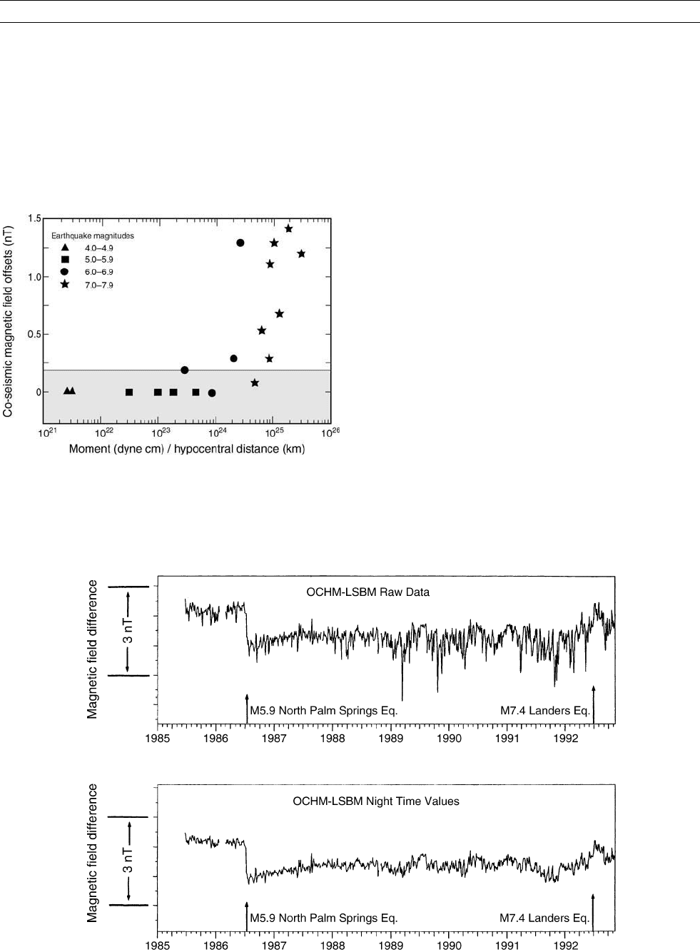
The primary features of seismomagnetic effects are shown in Figure S26

from Mueller and Johnston (1998). It is apparent that maximum signals

are not more than a nanotesla or so and these signals occur only for

larger earthquakes (M > 6) for which corresponding strain changes

are about a microstrain or so. An example of a magnetic record

observed at the epicenter of the 1986 M5.9 North Palm Springs earth-

quake and 17 km from the 1992 M7.4 Landers earthquake is shown in

Figure S27. For this, and some 40 other earthquakes with magnitude

between 5.5 and 7.4, no significant precursory magnetic signals were

observed.

Seismoelectric effects

Seismoelectric observations that show expected scaling with both

earthquake moment release and inverse distance cubed are difficult

to make because of the sensitivity of electrode contact potential to

earthquake shaking. Measurements of electrical resistivity to better

than 1% have been made since 1988 in a well designed experiment

installed near Parkfield, California (Park, 1997). An expected M6

earthquake together with several M5 earthquakes have occurred

beneath this array since 1990. None of these earthquakes generated

908 SEISMO-ELECTROMAGNETIC EFFECTS

any observable changes in resistivity above the measurement resolu-

tion (Park, 1997; Langbein et al., 2005).

Indirect observations of possible SE signals might be obtained using

the magnetotelluric (MT) technique to monitor apparent resistivity in

seismically active regions. Even with the best designed systems using

remote referencing systems to reduce noise and obtain stable impe-

dance tensors, it is difficult to reduce errors below 5% for good sound-

ings and 10–40% for poor soundings.

Possible high-frequency precurs ory effects

A number of observations purported to be high-frequency SEM effects

have been recently reported (Hayakawa, 1999). Interest in these higher

ULF frequencies primarily resulted from the fortuitous observation of

elevated ULF noise power on a single 3-component magnetometer

near the epicenter of the M7.1 Loma Prieta earthquake of October 18,

1989. However, similar records were not obtained with the 1992

M7.4 Landers earthquake, the 1994 M6.7 Northridge earthquake, the

1999 M7.1 Hector Mine earthquake, the 1999 M7.4 Izhmet, Turkey

earthquake and the 2004 M6 Parkfield, Ca, earthquake.

Though controversial, increased interest in tectonoelectric (TE) phe-

nomena related to earthquakes has resulted from suggestions in Greece

and Japan that short-term geoelectric field transients (SES) of particu-

lar form and character precede earthquakes with M > 5 at distances up

to several hundreds of kilometers. These transients appear to have a

spatially uniform source field on the scale of the array but no clear cor-

responding magnetic field transients and no sensible coseismic effects.

The SES have been empirically associated with subsequent distant

earthquakes and claimed as precursors (Varotsos et al., 1996).

Careful study of the SES recordings indicates that the SES signals

have the form expected from rectification/saturation effects of local

radio transmissions from high-power transmitters on nearby military

bases. Without any clear physical explanations describing how the

SES signals are earthquake generated yet coseismic effects related to

the much larger earthquake source are not observed, these observations

have been extremely controversial (Debate on VAN, 1996).

Another enigma concerns the generation of high-frequency (>1 kHz)

electromagnetic emissions associated with subsequent moderate earth-

quakes but, again, with no coseismic effects. Such emissions are

reported to have been detected at great distances from these earthquakes

(see summary by Hayakawa and Fujinawa, 1994) and by magnet-

ometers onboard satellites. However, the statistical significance of these

observations is under dispute.

The generation of high-frequency electromagnetic radiation can be

easily demonstrated in controlled laboratory experiments involving

Figure S26 Co-seismic magnetic field offsets as a function of

seismic moment scaled by hypocentral distance. The shaded

region shows the 2-sigma measurement resolution (from Mueller

and Johnston, 1998). Geodetically based seismomagnetic models

(Sasai, 1991) fit each offset.

Figure S27 Magnetic field differences between stations OCHM and LSBM before, during and after the July, 1986 M5.9 North Palm

Springs and the June, 1992 M7.4 Landers earthquakes (from Johnston et al., 1994).

SEISMO-ELECTROMAGNETIC EFFECTS 909

rock fracture in dry rocks. However, the Earth’s crust in seismically

active areas is quite conducting (0.3–0.001 S m

1

) and propagation

of very high-frequency (VHF) electromagnetic waves even short dis-

tances through the crust is difficult to justify physically. Propagation

from earthquake source regions (10–100 km in depth), and in some

cases through oceans with conductivities of 1 S m

1

, is physically

implausible. More significantly, the amount of allowable rock fractur-

ing prior to earthquakes is strongly constrained by high sensitivity

crustal strain measurements in the near-field of many earthquakes.

These measurements indicate moment release (m  slip  area) prior

to earthquakes is at least three orders of magnitude smaller than that

released at the time of an earthquake (Johnston and Linde, 2002).

Appeal to secondary sources at the Earth’s surface may avoid this

difficulty but the expected associated near-field crustal strain and

displacement fields are not observed.

High-frequency disturbances are generated in the ionosphere as a

result of coupled infrasonic waves generated by earthquakes and are

readily detected with routine ionospheric monitoring techniques and

global position system (GPS) measurements. In essence, displacement

of the Earth’s surface by an earthquake acts like a huge piston, gener-

ating propagating pressure waves in the atmosphere/ionosphere wave-

guide. Thus, traveling waves in the ionosphere (traveling ionospheric

disturbances or TIDs) are a consequence of earthquakes (and volcanic

eruptions). EM data at VHF frequencies recorded on ground receivers

or by satellite require correction for TID and other disturbances before

any association can be made to source processes or earthquake

precursors.

Malcolm J.S. Johnston

Bibliography

Debate on VAN, 1996. Special issue. Geophysical Research Letters,

23: 1291–1452.

Hayakawa, M. (ed.), 1999. Atmospheric and Ionospheric Electromag-

netic Phenomena Associated with Earthquakes. Tokyo: Terra

Scientific Publishing Company, p. 996.

Hayakawa, M., and Fujinawa, F. (eds.), 1994. Electromagnetic Phe-

nomena Related to Earthquake Prediction. Tokyo: Terra Scientific

Publishing Company, p. 677.

Johnston, M.J.S., 2002. Electromagnetic fields generated by earth-

quakes. International Handbook of Earthquake and Engineering

Seismology, Volume 81A. New York: Academic Press, pp. 621–635.

Johnston, M.J.S., and Linde, A.T., 2002. Implications of crustal strain

during conventional, slow and silent earthquakes. International

Handbook of Earthquake and Engineering Seismology, Volume

81A. New York: Academic Press, pp. 589– 605.

Johnston, M.J.S., Mueller, R.J., and Sasai, Y., 1994. Magnetic field

observations in the near-field of the 28 June 1992 M7.3 Landers,

California, earthquake. Bulletin of the Seismological Society of

America, 84: 792–798.

Langbein, J., Borcherdt, R., Dreger, D., Fletcher, J., Hardebeck, J.L.,

Hellweg, M., Ji, C., Johnston, M., Murray, J.R., Nadeau, R.,

Rymer, M., and Treiman, J., 2005. Preliminary report on the 28

September 2004, M 6.0 Parkfield, California earthquake. Seismolo-

gical Research Letters, 76:10–26.

Mueller, R.J., and Johnston, M.J.S., 1998. Review of magnetic field

monitoring near active faults and volcanic calderas in California:

1974–1995. Physics of the Earth and Planetary Interiors, 105 :

131–144.

Park, S.K., 1997. Monitoring resistivity change in Parkfield,

California: 1988–1995, Journal of Geophysical Research, 102:

24545–24559.

Reid, H.F., 1914. Free and forced vibrations of a suspended magnet.

Terrestrial Magnetism, 19:57–189.

Rikitake, T., 1966. Elimination of non-local changes from total inten-

sity values of the geomagnetic field. Bulletin of Earthquake

Research Institute, 44: 1041–1070.

Sasai, Y., 1991. Tectonomagnetic modeling on the basis of linear

piezomagnetic effect. Bulletin of the Earthquake Research Insti-

tute, 66: 585–722.

Varotsos, P., Eftaxias, K., Lazaridou, M., Nomicos, K., Sarlis, N.,

Bogris, N., Makris, J., Antonopoulos, G., and Kopanas, J., 1996.

Recent earthquake predictions results in Greece based on the obser-

vation of seismic electric signals. Acta Geophysica Polonica, 44:

301–307.

Cross-references

Geomagnetic Spectrum, Temporal

Gravity-Inertio Waves and Inertial Oscillations

Magnetotellurics

Volcano-Electromagnetic Effects

SHAW AND MICROWAVE METHODS,

ABSOLUTE PALEOINTENSITY DETERMINATION

The Shaw technique is used to determine the strength of the Earth ’s

magnetic field from igneous rocks and man fired artifacts. In this tech-

nique (Shaw, 1974) the natural remanent magnetization (NRM) of the

sample is demagnetized using alternating field (AF) demagnetization

but is remagnetized by heating to above the Curie temperature and

cooling in a known field to form a full thermoremanent magnetization

(TRM) in a known field strength. By comparing the NRM and TRM

values it is possible to calculate the strength of the field in which the

NRM was formed. There are checks for alteration of the sample and

also several variations of the original technique that are described

below.

The original Shaw technique

This technique used anhysteretic remanent magnetizations (ARMs) to

check for any alteration in the sample due to the laboratory heating.

There are four demagnetization stages to the experiment:

1. AF demagnetize the NRM in steps to a maximum AF value.

2. Give the sample an ARM in a known constant field in the maxi-

mum AF used in 1 (ARM1) and AF demagnetize in the same steps

used in 1.

3. Give the sample a full TRM in a known constant laboratory field

strength and AF demagnetize in the same steps used in 1.

4. Give the sample an ARM in the same known field as used in 2

(ARM2) and AF demagnetize in the same steps used in 1.

The basic premise is simply that if a sample can be demagnetized

between two AF values then it can also be remagnetized with an

ARM between those values. The value of the ARM is not simply

related to the value of the NRM (or TRM) lost between those AF

values but it is a function of the samples’ ability to retain magnetiza-

tion between those two AF values. If the sample becomes altered dur-

ing heating to form the TRM in such a way that the ability to retain

magnetization (TRM or ARM) between those two values changes,

then the value of ARM2 (given after heating) between the two AF

values will be different from the value of ARM1 (which was given

before heating and, therefore, before alteration).

By plotting the demagnetization values of ARM1 against ARM2

and using the value of the AF demagnetizing field as a parameter,

the slope of the line should be unity if there has been no alteration

of the sample. If there has been alteration, then the slope will not be

unity. By selecting the continuous AF demagnetization region where

the slope is unity (if such a region exists) and plotting NRM against

TRM it is possible to calculate the ratio NRM/TRM (Figure S28)

910 SHAW AND MICROWAVE METHODS, ABSOLUTE PALEOINTENSITY DETERMINATION

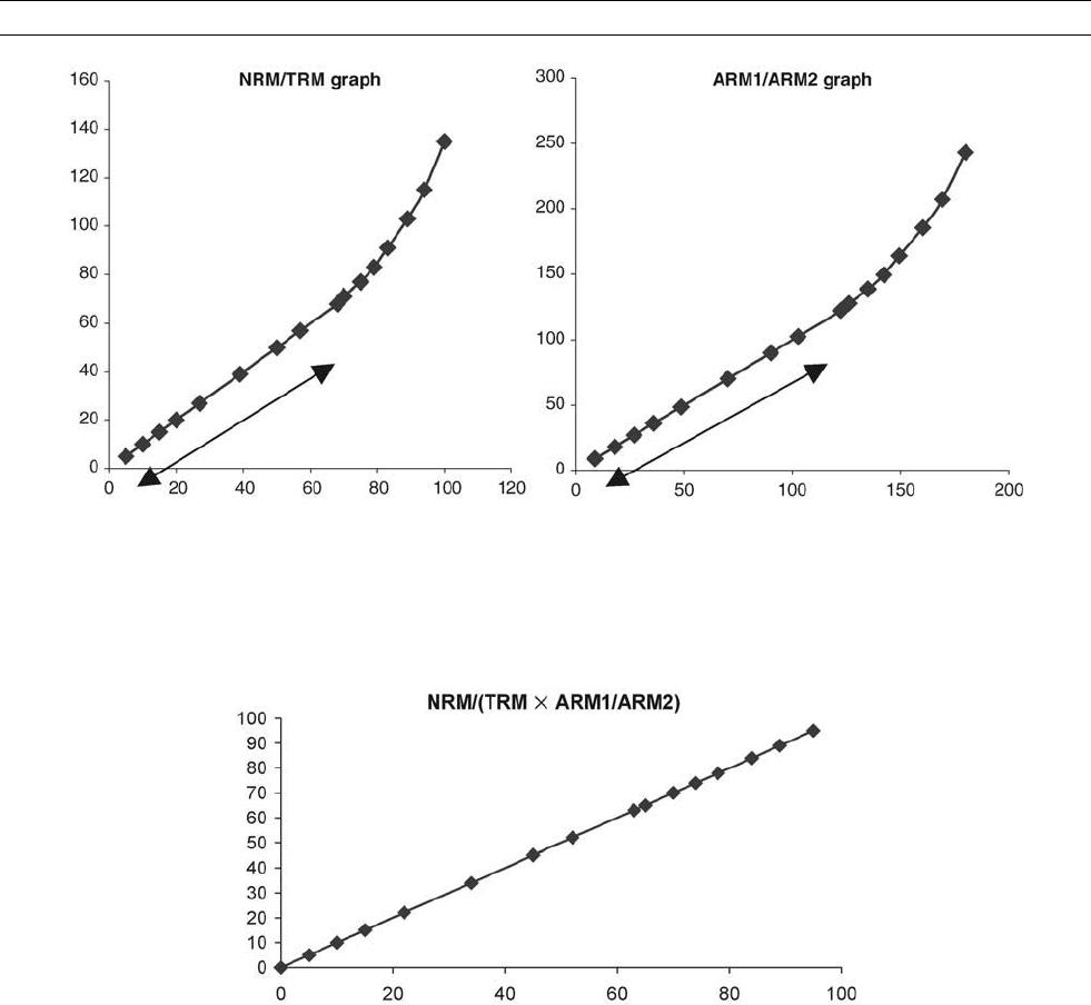
which is the same ratio as the ancient field strength/laboratory field

strength (Nagata, 1943).

Kono, and Rolph and Shaw corrections

Kono (1978) proposed that samples with altered TRMs could be

used for paleointensity analysis provided that the NRM/TRM graph

has a linear segment and that the equivalent ARM1/ARM2 graph is

also linear. He proposed multiplying the paleointensity obtained from

the NRM/TRM linear section by the inverse of the slope of the equiva-

lent ARM1/ARM2 section in order to correct for laboratory thermal

alteration.

Rolph and Shaw (1985) proposed that the degree of alteration of the

TRM was reflected in the degree of alteration of ARM2 and so it

should be possible to use the ARM data to continuously correct for

alteration in the TRM. In order to achieve this, the final highest AF

field value of NRM, TRM, ARM1, and ARM2 are subtracted from

their respective data. Each TRM value is then multiplied by the ratio

of ARM1/ARM2 for the same AF value. A new graph plotting

NRM against TRM  ARM1/ARM2 should correct for any alteration

of the TRM due to laboratory heating (Figure S29).

Double heating technique

Following on from the Rolph and Shaw correction, Tsunakawa and

Shaw (1994) applied a second heating to form a second TRM

(TRM2) in the same field as the first TRM (TRM1). If both the first

and second heatings cause thermal alteration, then it is possible to

check if the ARM correction proposed by Rolph and Shaw works by

plotting TRM1 against ARM corrected TRM2. The slope of the line

should be unity if the correction works. This adaptation of the Shaw

technique is lengthier because of the need for two heatings and a third

set of ARM measurements but it gives confidence to final result if the

TRM2 correction works.

Figure S28 Shaw technique paleointensity analysis, the high AF region of the ARM1/ARM2 graph is linear with slope 1 (marked with

double ended arrow). The same AF region on the NRM/TRM graph is also linear and as this AF region is unaltered the paleointensity

value can be calculated from the slope.

Figure S29 The data in this figure analyzed using the Rolph and Shaw correction where changes in ARM are used to correct for changes

in TRM. In the Rolph and Shaw technique only data with peak AF values above 0.1 T were used in order to restrict the analysis to single

or pseudosingle domain grains.

SHAW AND MICROWAVE METHODS, ABSOLUTE PALEOINTENSITY DETERMINATION 911

Low temperat ure demagnetization double heating

technique

Tsunakawa et al. (1997) and Yamamoto et al. (2003) used low tem-

perature demagnetization (LTD) in conjunction with the double heat-

ing technique. The low temperature demagnetization (to liquid

nitrogen temperature) removed the magnetization formed during high

temperature oxidation of the magnetic grains. Although the technique

is lengthy, it has provided accurate paleointensity determinations from

recent Hawaiian lavas.

John Shaw

Bibliography

Kono, M., 1978. Reliability of palaeointensity methods using alternat-

ing field demagnetization and anhysteretic remanence. Geophysical

Journal of Royal Astronomical Society, 54: 241–261.

Nagata, T., 1943. The natural remnant magnetism of volcanic rocks

and its relation to geomagnetic phenomena. Bulletin of the Earth-

quake Research Institute, 21:1–196.

Rolph, T.C., and Shaw, J., 1985. A new method of palaeofield magni-

tude correction for thermally altered samples and its application

to Lower Carboniferous lavas. Geophysical Journal of Royal

Astronomical Society, 80: 773–781.

Shaw, J., 1974. A new method of determining the magnitude of the

palaeomagnetic field. Application to five historic lavas and five

archaeological samples. Geophysical Journal of Royal Astronomi-

cal Society, 39: 133–144.

Tsunakawa, H., and Shaw, J., 1994. The Shaw method of palaeointen-

sity determination and its application to recent volcanic rocks.

Geophysical Journal International, 118: 781–787.

Tsunakawa, H., Shimura, K., and Yamamoto, Y., 1997. Application of

Double Heating Technique of the Shaw Method to the Brunhes

Epoch Volcanic Rocks. 8th Scientific Assemble of IAGA.

Yamamoto, Y., Tsunakawa, H., and Shibuya, H., 2003. Palaeointensity

study of the Hawaiian 1960 lava: implications for possible causes

of erroneously high intensities. Geophysical Journal International,

153: 263–276.

Cross-references

Demagnetization

Magnetization, Natural Remanent (NRM)

Magnetization, Thermoremanent (TRM)

SHOCK WAVE EXPERIMENTS

Introduction and background

Shock wave experiments have a special place in the study of the

Earth’s interior and the interiors of the terrestrial planets because vir-

tually the entire pressure (to 470 GPa) and temperature (to 6000 K)

ranges existing with these objects can be achieved, via this technique,

in the laboratory. The study of the properties of iron and alloys, solid

and molten, relevant to core composition via shock compression to

high pressures and temperatures of the Earth and planetary cores has

continued to challenge mineral physicists.

The geomagnetic field is thought to be generated by complex con-

vective flows of electrically conducting Fe-rich fluids in the fluid outer

core. The author has measured physical properties under shock com-

pression which provide information on where possible Fe-rich materi-

als are fluid and, hence, where convection and generation of the

geomagnetic field occurs.

Dynamic compression of cosmochemically candidate metal-like

compounds which, in the molten state, are soluble in molten iron such

as FeS, FeO, FeC, FeSi, and FeH

continue to be of interest to theories

of the formation and evolution of the molten conductive cores that

generates the Earth’s and other planetary magnetic fields (see Core

composition). The electrical resistivity of iron alloys and compounds

under shock compression are compared to approximate bounds for

the Earth that are derived theoretically. Recent compositional and ther-

modynamic models of the Earth’s core (see Core, adiabatic gradient)

have been strongly revised (Anderson and Ahrens, 1994; Poirier,

1994; Stacey, 2001; Anderson and Isaak, 2002) in part, on account

of new shock wave data for iron and its alloys.

Here we present a summary of modern techniques for shock wave

equation of state (EOS) (pressure-volume-energy) measurements

which are applicable to condensed matter, in general, and specific to

iron and its alloys. The study of compression behavior of other stan-

dard materials and phase transitions in selected materials have pro-

vided standards for the more widely used diamond and multianvil

high pressure apparatuses (Holzapfel, 1996). Improvements in techni-

ques for measuring sound, or rarefaction velocity in shock-compressed

material (Brown and McQueen, 1986; McQueen, 1992; Chen and

Ahrens, 1998) have continued to complement the EOS measurements

for these materials and provide data specifying whether materials in

various shock states are in solid, partially or completely molten form.

Such data also provide firm constraints on the high-pressure and

high-temperature Grüneisen parameter of iron and iron alloys (see

Grüneisen’s parameter for iron and Earth’s core). As discussed

below, knowledge of the Grüneisen ratio of iron is crucial to reducing

shock wave data to pressure-volume isotherms and isentropes so that

it may be compared to data from other sources, as well as to constrain

the thermodynamic models of the Earth’s core.

Shock wave generation and the Rankine-Hugoniot

equation

The shock waves used for dynamic compression research must be

maintained for time intervals of 10

times the intrinsic rise-time t

of the shock front (Figure S30).

The impact of gun and explosively launched flyer plates both pro-

vide the requisite nearly steady waves in materials. For steady waves,

a shock, with velocity U with respect to the laboratory, independent of

time, can be defined and conservation of mass, momentum, and energy

across a shock front can be expressed as:

¼ r

U=ðU  u

Þ; (Eq. 1)

¼ r

U; (Eq. 2)

 E

¼ P

ð1=r

 1=r

Þ=2 ¼ 1=2u

; (Eq. 3)

where r, u, P, and E are density, particle velocity, shock pressure, and

internal energy and, (as indicated in Figure S31), the subscripts 0 and 1

refer to the state in front of and behind the shock front, respectively. It

should be understood that in this section, pressure is used in place of

stress in the indicated wave propagation direction. Actually stress, in

the wave propagation direction, is what is specified by (2). A detailed

derivation of (1) –(3) is given in Melosh (1989). Equation (3) also indi-

cates that the material achieves an increase in internal energy (per

unit mass) which is exactly equal to one-half of the kinetic energy

per unit mass.

Upon driving a shock of pressure P

into a material, a final shock

state is achieved which is described by (1)– (3). This shock state is

shown in relation to other thermodynamic paths in Figure S32 in the

pressure-volume plane. Here V

¼ 1/r

and V ¼ 1/r. In the case of

the isotherm and isentrope, it is possible to follow, as a thermodynamic

path, the actual isothermal or isentropic curve to achieve a state on the

isotherm or isentrope. A shock or Hugoniot state is different, however.

912 SHOCK WAVE EXPERIMENTS

The Hugoniot state P

, V

is achieved via a thermodynamic path given

by the straight line called Rayleigh line (Figure S32). Thus successive

states along the Hugoniot curve cannot be achieved, one from another,

by a shock process. The Hugoniot curve itself then just represents the

locus of final shock states.

To achieve such shock waves with flat-topped stress pulses, flat

plates called flyer plates are launched with guns (Figure S33) or explo-

sive devices (Figures S34 and S35). The flyer plate impacts the sample

or a “driver plate” upon which the sample is mounted and drives a

shock into the driver plate and the sample. Although the various plate

launching systems depicted in Figures S33–S35 operate over an enor-

mous velocity range, all actual systems have shortcomings. Correc-

tions for converging flow must be made in the case of explosive

imploding systems of Figure S35. Tilt and flyer plate distortion, must

be taken into account in the case of all explosive and gun launched

impactors, as for example, indicated in Figure S36.

Comparison of electrical resistivity of shocked iron,

iron alloys, and compounds to Earth

Our understanding of the conditions required to generate the Earth’s

magnetic field provides some constraints on the electrical conductivity

of the Earth which may be usefully compared to the conductivity of

Figure S30 Generation of shock waves by flyer plate impact.

Impact induces steady flat-topped shock wave and this is followed

by a rarefaction wave (from Ahrens (1987)).

Figure S31 Profile of a steady shock wave, rise time t

, imparting

a particle velocity u

, pressure P

, density r

, and internal energy

density E

, propagating with velocity U into material that is

at rest at density r

and internal energy density E

(from

Ahrens (1987)).

Figure S32 Pressure-volume compression curves. For isentrope

and isotherm, the thermodynamic path coincides with the locus

of states, whereas for the shock, the thermodynamic path is a

straight line (from point 0, V

) to point (P

, V

) on the Hugoniot

curve (from Ahrens (1987)).

Figure S33 Diagrams of propellant gun launching system to

impact metallic targets up to 2.6 km s

1

. The iron target is

preheated with radiofrequency induction coils. Resulting target

temperature is monitored using the optical signal reflected from

gold mirror (M). Abbreviations: W: window; L: lens; M: mirror;

M (Au): gold mirror; T: EOS turning mirror. About 1 s before

launching projectile, EOS turning mirror is inserted in front of the

target free-surface (after Chen and Ahrens (1998)).

SHOCK WAVE EXPERIMENTS 913

solid and molten iron and alloys as a function of temperature

and pressure.

The resistivity of the Earth’s core is thus constrained to be suffi-

ciently low, such that magnetic field lines and unable to diffuse out

of the core on the timescale of 10

years approximately obtained

by assuming radius of the core (usually assumed to be the inner core)

(1200 km), divided by the westward drift velocity (of features of the

magnetic field such as mapped by Bloxham and Gubbins (1985) from

the years 1715 to present). Using this loose constraint, Matassov

(1977) first showed that the core should have a resistivity of

r < 10

5

 10

4

O m: (Eq. 4)

These low resistivity values assume that the magnetic field will not

diffuse out of the core over the 10

year time scale field deflation.

By assuming a fixed value of 8–12% of the total Earth heat flow

(44 TW) across core-mantle boundary, a lower limit resistivity of

the core region of

r < 10

6

O m (Eq. 5)

is obtained. This rather simple constraint limit is obtained by taking

the extreme assumption that the heat flow across the CMB is totally

resulting from ohmic heating by the core of the geodynamo.

As can be seen in Figure S37, upon extrapolation, the mostly

lower pressure shock data for iron, and its alloys and compounds

to 135–450 GPa, the resistivity of these media lies in the

–6

–10

–5

Ωm range in agreement with the very loose theoretical

expectations described above.

At least three sources of energy for powering the geodynamo are

recognized:

1. Hydrodynamic flow of core fluid induced by the difference in

dynamic ellipticity of the whole Earth versus that of the core.

2. Thermal convection of core fluid driving the geomagnetic dynamo

also appears possible. Such thermal convection could be driven by

radioactivity of the core, such as for example, supplied by

Kin

the core.

3. Another source of sufficient thermal energy to operate the geody-

namic dynamo is the latent heat of crystallization of the inner, solid

core.

Shock wave equation of state (EOS) measurements

In the simplest case when a single shock state is achieved via a shock

front, the Rankine-Hugoniot equations involved six variables (U, u

, r

, E

–E

, and P

); thus, measuring three, usually U, u

, and r

determines the shock state, r

, E

–E

, and P

Figure S34 Explosive flyer plate launching (to 5kms

1

)

apparatus. (1) and (2) Explosive plane-wave lens is point detonated

at upper (downwards pointing) arrow. (1) Fast detonating explosive,

(2) slow detonating explosive, (3) main explosive. (8) Plexiglas buffer

plate, (4) metal flyer plate, (5) driver plate, (6) specimens under

study, (7) electrical contactor pin switches that detect shock wave

arrival (after Al’tshuler et al. (1999)).

Figure S35 Hemispheric implosive flyer plate launching

devices for ultra-high pressure shock wave research. (a) Single

stage apparatus launches metal flyer plates to velocities of

9–11 km s

1

. (b) Explosive charge is multiply point detonated

at outer surface of explosive hemisphere. (1) Main charge,

(2) hemispherical primary flyer plate. Upon acceleration of

primary flyer plate to 5–7 km s

1

impact onto (6) secondary

explosive charge induces an overdriven detonation wave.

Overdriven detonating wave in secondary charge accelerates

(7) secondary flyer plate to velocities of up to 14 km s

1

. Upon

impact onto (3) driver plate, shock waves with pressures in

1400–1800 GPa are driven into (4) specimens. Resulting shock

velocities are measured via (5) electric contactor pin switches

(after Al’tshuler et al. (1999)).

914 SHOCK WAVE EXPERIMENTS

Careful measurement of sample volumes and mass can result in r

to be determined within 0.3%. Projectile or flyer plate velocity is

measured via successive closure of a series of contactor pin switches

or via optical or flash X-ray techniques (Ahrens, 1987). In the simplest

case where the sample and impactor are made of the same material, the

shock-induced particle velocity is

¼ u

=2; (Eq. 6)

where u

is the flyer plate velocity which is measured to 0.5%.

Shock velocity is usually measured to 1% via streak camera

photography (Figures S33 and S36) or via contactor pin closures

(Figures S34 and S35) as indicated.

Shock compression data for candidate core constituents are tabu-

lated by Ahrens and Johnson (1995). Upon shock compression to

greater than 13 GPa, the Hugoniot data for iron demonstrates the onset

of a 5% volume decrease upon transition from the low pressure, bcc,

a-phase to the high pressure hcp, e-phase. Moreover, the phase change

demonstrates hysteretic unloading (for example, as seen from 23 GPa

shown in Figure S38). The shock wave data for iron (up to 200 GPa

were originally obtained using explosively launched flyer plates,

Figure S34) and extended to 900, and later, 1400 GPa using the

techniques sketched in Figures S35a and b by Al’tschuler and

co-workers in the former Soviet Union (now Russia) (Ahrens and

Johnson, 1995). Shock wave data for Fe-Si (Matassov, 1977),

pyrrhotite (FeS) (Brown et al., 1984), pyrite (FeS

) (Ahrens and

Jeanloz, 1987), and wüstite (FeO) (Jeanloz and Ahrens, 1980) may

be used to estimate the fraction of light elements in the core by correct-

ing Hugoniot temperatures to those of the Earth (as for example as

shown in Figures S39 and S44) (see Inner Core composition and Core

temperature).

Strategy for applying shock wave data to modeling

the Earth’s core

Theoretical temperature model s of the Earth’s core

Thermal models of the outer core of the Earth have been anchored to

estimates of the pure iron melting point at 330 GPa, the pressure of the

inner core-outer core (IC-OC) boundary (see Melting temperature of

iron in the core, theory and Melting temperature of iron in the core,

experimental ). Since the temperature variation T

¼ T

(g/V

)in

the outer core (which is assumed to be in approximately adiabatic

equilibrium) is usually modeled as an isentropic temperature distribu-

tion which is described by (see Core, adiabatic gradient):

¼ T

icoc

exp 

icoc



: (Eq. 7)

Here g is the Grüneisen parameter of the molten material of the outer

core (usually assumed to be approximately equal to that of molten

Figure S36 (Upper) Schematic illustration (highly exaggerated) of projectile tilt and bowing, and their effect on the streak record.

Particle-velocity vector (up) is normal to target (seen edge-on) despite tilt. The arrival on the streak record corresponding to the

shock-wave entering the sample could significantly be curved due to the bowing of the projectile (after Jeanloz and Ahrens (1980)).

(Lower) (a) Experimental sample image taken through image converter camera, viewing the back-side of the target. The sample and

mirror can be seen, as well as the location of the slit. (b) Streak photograph taken by sweeping the image of the slit towards the

right (at nearly constant velocity) as the projectile impacted the target. Note the intense flash of light as the shock-wave crosses the

sample/buffer mirror interface (after Jeanloz and Ahrens (1978)).

SHOCK WAVE EXPERIMENTS 915