Graebel W.P. Advanced Fluid Mechanics
Подождите немного. Документ загружается.

64 Inviscid Irrotational Flows
Remembering that the circulation of the image vortex is reversed, from equation (2.2.19)
the velocity potential for the original vortex plus its image is
total
=
orig
+
image
=10
tan
−1
y −1
x
−tan
−1
y +1
x
Taking the gradient of the velocity potential, the velocity components are found to be
v
x
=10
−y −1
x
2
+y −1
2
+
y +1
x
2
+y +1
2
v
y
=10
x
x
2
+y −1
2
−
x
x
2
+y +1
2
The induced velocity at (0, 1, 0) is the velocity at that point due to the image vortex.
This gives a velocity at (0, 1, 0) of v
x
= 10 ·2/2
2
= 5m/sv
y
= 0. The vortex thus
moves parallel to the wall at a speed of 5 m/s.
Example 2.2.3 A vortex pair in a cup
A vortex pair is generated in a cup of coffee of radius c by brushing the tip of a
spoon lightly across the surface of the coffee. The pair so generated will have opposite
circulations (try it!). If the vortex with positive circulation is at a b, and the vortex
with negative circulation at a −b, verify that the flow with the cup is generated by
an image vortex with positive circulation at ac
2
/a
2
+b
2
−bc
2
/a
2
+b
2
, plus an
image vortex with negative circulation at ac
2
/a
2
+b
2
bc
2
/a
2
+b
2
. These image
points are located at what are called the inverse points of our cup.
Solution. What is needed is a pair of opposite-rotating vortices plus the images
needed to generate the cup. Each vortex moves because of the induced velocity generated
by the images and the other vortex. The given vortex pair has a stream function
=−
4
lnx −a
2
+y −b
2
−lnx −a
2
+y +b
2
=−
4
ln
x −a
2
+y −b
2
x −a
2
+y +b
2
The proposed stream function consists of the original stream function plus the stream
function due to a pair of vortices at ak bk and ak −bk, where k = c
2
/a
2
+b
2
.
The combined stream function is then
=−
4
lnx −a
2
+y −b
2
−lnx −a
2
+y +b
2
+lnx −ak
2
+y −bk
2
−lnx −ak
2
+y +bk
2
As a check of the result, on the circle of radius c
x = c cos and y = c sin and so
=−
4
lnc cos −a
2
+c sin −b
2
+lnc cos −ak
2
+c sin +bk
2
−lnc cos −a
2
+c sin +b
2
−lnc cos −ak
2
+c sin −bk
2
.
2.2 Irrotational Flows and the Velocity Potential 65
But since cos
2
+sin
2
= 1 and using the definition of k
c cos −ak
2
+c sin −bk
2
=c
2
−2ka cos +b sin +a
2
+b
2
k
2
=kc
2
/k −2a cos +b sin +a
2
+b
2
k
=ka
2
+b
2
−2a cos +b sin +c
2
=kc cos −a
2
+c sin −b
2
and
c cos −ak
2
+c sin +bk
2
=c
2
−2ka cos −b sin +a
2
+b
2
k
2
=kc
2
/k −2a cos −b sin +a
2
+b
2
k
=ka
2
+b
2
−2a cos −b sin +c
2
=kc cos −a
2
+c sin +b
2
Substituting these into the expression of the stream function, we have
=−
4
lnc cos −a
2
+c sin −b
2
+ln kc cos −a
2
+c sin +b
2
−lnc cos −a
2
+c sin +b
2
−ln kc cos −a
2
+c sin −b
2
=0
Thus, the cup of radius c is a streamline with the stream function equal to zero.
To find the equations that govern how the vortex at a b moves, the induced
velocity components are computed by taking the derivatives of , omitting the term
from the vortex at (a, b), and then letting x = a y =b. The result is
a =
b
2
1
2b
2
−
a
2
+b
2
a
2
+b
2
+c
2
a
2
a
2
+b
2
−c
2
2
+b
2
a
2
+b
2
+c
2
2
+
1
a
2
+b
2
−c
2
,
b =
a
2
a
2
+b
2
a
2
+b
2
+c
2
a
2
a
2
+b
2
−c
2
2
+b
2
a
2
+b
2
+c
2
2
−
1
a
2
+b
2
−c
2
.
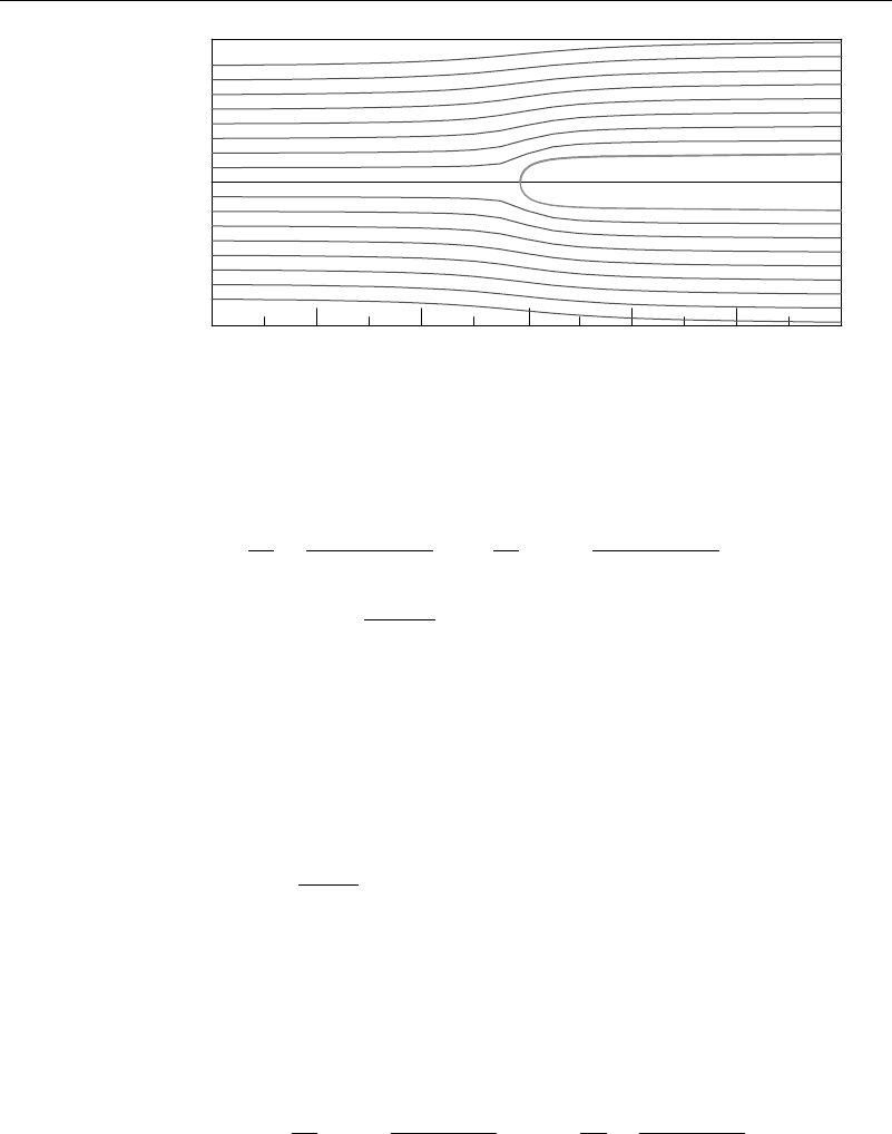
2.2.7 Rankine Half-Body
A source located at the origin in a uniform stream (Figure 2.2.9) has the velocity
potential and a stream function
=xU +
m
2
ln
x
2
+y
2
= yU +
m
2
tan
−1
y
x
(2.2.41)
in a two-dimensional flow, and
=zU −
m
4
√
r
2
+z
2
=
1
2
r
2
U −
m
4
√
r
2
+z
2
(2.2.42)
in a three-dimensional flow.
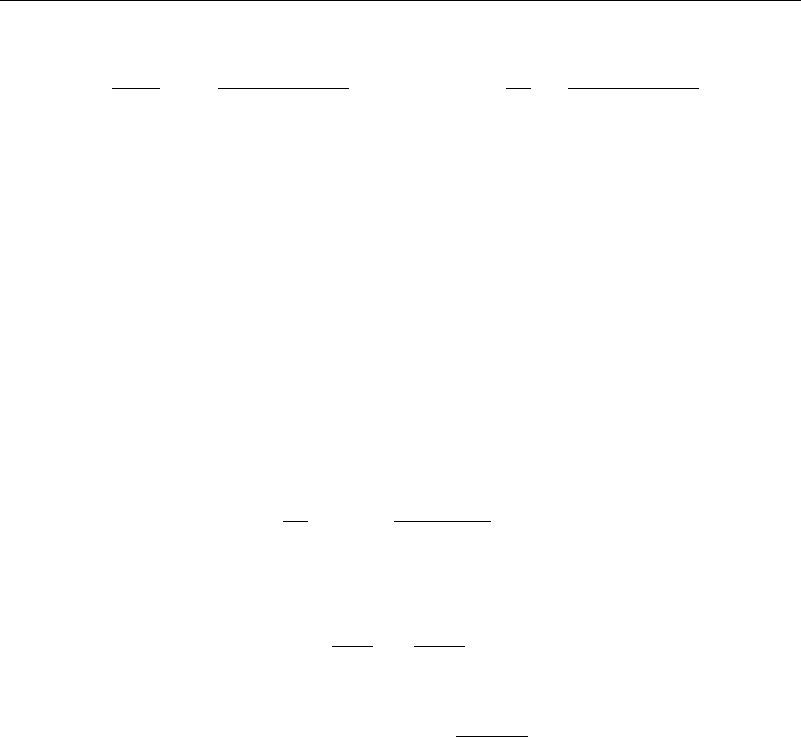
66 Inviscid Irrotational Flows
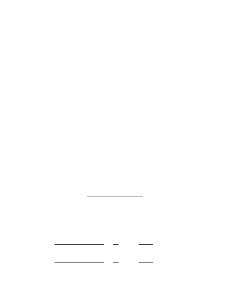
2.0
1.0
0.0
Y
X
–1.0
–2.0
–6 –4 –2 0 2 4 6
Figure 2.2.9 Rankine half-body—two dimensions
Examining the three-dimensional case in further detail, we find the velocity com-
ponents to be
v
r
=
r
=
mr
4r
2
+z
2
3/2
v
z
=
x
=U +
mz
4r
2
+z
2
3/2
(2.2.43)
It is seen from equation (2.2.43) that there is a stagnation point v
stagnation point
=0
at the point r = 0z =−
√
m/4U.Onr = 0, the stream function takes on values
=−m/4 for z positive and = m/4 for z negative. The streamline = m/4
goes from the source to minus infinity. At the stagnation point, however, it bifurcates
and goes along the curve z
2
= b
2
−2r
2
2
/4b
2
−r
2
z
2
= b
2
−2r
2
2
/4b
2
−r
2
with
b
2
=m/U . This follows by putting = m/4 into equation (2.2.42) and solving for
z. The radius of the body goes from 0 at the stagnation point to r
=b far downstream
from the source. This last result can be obtained either from searching for the value
of r needed to make z become infinite in equation (2.2.43) or by realizing that far
downstream from the source the velocity must be U and all the discharge from the source
must be contained within the body. In either case, the result is that far downstream the
body radius is b =
√
m/U.
This flow could be considered as a model for flow past a pitot tube of a slightly
unusual shape. A pitot tube determines velocity by measuring the pressure at the stagna-
tion point and another point far enough down the body so that the speed is essentially U.
The difference in pressure between these two points is proportional to U
2
. This pressure
difference can be found from our analytical results by writing the Bernoulli equation
between the stagnation point and infinity.
In the two-dimensional counterpart of this, the velocity is
v
x
=
x
=U +
mx
2x
2
+y
2
v
y
=
y
=
my
2x
2
+y
2
with the stagnation point located at −m/2U 0 .Ony =0=0 for x positive and
m/2 for x negative. The streamline =m/2 starts at − 0, going along the x-axis to
the source. At the stagnation point the streamline bifurcates, having the shape given by
2Uy/m = −tan
−1
y/x (2.2.44)
The asymptotic half-width of the body is y
=m/2U .
2.2 Irrotational Flows and the Velocity Potential 67
It is instructive to examine the behavior of the and lines at the stagnation point.
For the two-dimensional case, first expand about the stagnation point in a Taylor
series about −m/2U 0 , giving to second order in x +m/2U and y
=
m
2
−
4U
2
m
x +
m
2U
y +···
This tells us that at the bifurcation point, the = m/2 line is either along y = 0or
perpendicular to it (i.e., locally either on y =0oronx =−m/2U.
Expanding about −m/2U 0 to second order in x +m/2U and y, we have
=
m
2
−1+ln
m
2U
+
2U
2
m
−
x +
m
2U
2
+y
2
+···
This tells us that =
m
2
−1+ln
m
2U
along lines with slope ±45
y =±x +m/2U
,
thereby bisecting the lines as we had earlier expected would happen.
Notice that if we wish to model this flow on a Hele-Shaw table, one way of
accomplishing this without the necessity of drilling any holes in our table would be to
cut out a solid obstacle of the shape given by setting = m/2 and then placing it on
the table aligned with the flow. The flow exterior to the obstacle is the same as if we
had drilled a hole and inserted the source.
2.2.8 Rankine Oval
The previous Rankine half-body was not closed because there was a net unbalance in
mass discharge. By putting an aligned source and sink pair in a uniform stream with
the source upstream of the sink, a closed oval shape is obtained. The velocity potential
and stream function then become
=xU +
m
2
ln
x +a
2
+y
2
−ln
x −a
2
+y
2
= yU +
m
2
tan
−1
y
x +a
−tan
−1
y
x −a
(2.2.45)
for a two-dimensional body, and
=zU +
m
4
1
r
2
+z +a
2
−
1
r
2
+z −a
2
=
1
2
r
2
U +
m
4
z +a
r
2
+z +a
2
−
z −a
r
2
+z −a
2
(2.2.46)
for a three-dimensional body.
The velocity for the two-dimensional body is
v
x
=
x
=U +
m
2
x +a
x +a
2
+y
2
−
x −a
x −a
2
+y
2
v
y
=
y
=
m
2
y
x +a
2
+y
2
−
y
x −a
2
+y
2
The stagnation points are therefore at ±
a
2
+ma/U 0.
68 Inviscid Irrotational Flows
For the two-dimensional case, according to equation (2.2.45) the streamline that
makes up the body is given by = 0. (Notice that along y = 0= 0, except in the
range −a<x<a, where =−m/2.) Therefore, the equation giving the body shape is
0 = yU +
m
2
tan
−1
y
x +a
−tan
−1
y
x −a
(2.2.47)
From symmetry, the maximum height of the body will be at x =0. This height is given
from equation (2.2.47) as a solution of the equation
y
max
=
m
2U
−2tan
−1
y
max
a
(2.2.48)
Similar results hold for the three-dimensional case. The parameter governing shape
is m/Ua in the two-dimensional case and m/Ua
2
in the three-dimensional case. If m/Ua
is large, the body is long and slender. If m/Ua is small, the body is short and rounded.
More complicated Rankine ovals can be formed by putting more sources and sinks
in a uniform stream. For the body to close, it is necessary that the sum of the source
and sink strengths be zero. This, however, is not a sufficient condition. Notice that in
our simple example that if the source and sink were interchanged (just change the sign
of m), there will be no closed streamlines about the source and sink pair.
2.2.9 Circular Cylinder or Sphere in a Uniform Stream
The Rankine oval is an unfamiliar geometrical shape, but if you plot its shape for various
values of the separation a and the shape parameter m/Ua, you can see that as the
source-sink pair get closer together while the shape parameter is held constant, the oval
shape becomes more and more circular. This suggests that in the limit as the source-sink
pair becomes a doublet, a circular shape would be achieved. The source portion of the
doublet should be facing upstream and the sink portion facing downstream in order to
generate a closed stream surface.
The velocity potential and stream function for a uniform stream plus a doublet is
=xU +
xB
x
x
2
+y
2
=yU −
yB
y
x
2
+y
2
(2.2.49)
in a two-dimensional flow, and
=zU +
zB
z
r
2
+z
2
3/2
=
1
2
r
2
U −
r
2
B
z
r
2
+z
2
3/2
(2.2.50)
in a three-dimensional flow.
If we let B
x
=Ub
2
in the two-dimensional case, equation (2.2.50) shows that =0
both on y = 0 and on x
2
+y
2
=b
2
. Therefore, we have flow past a circular cylinder of
radius b. Letting B
z
=Ub
3
/2 in three dimensions gives = 0 on a sphere of radius b.
How does this solution relate to the method of images? The interpretation is com-
plicated by having to consider a curved mirror, but the flow can be thought of as the
body that focuses the uniform stream upstream (a very large distributed source) into the
source part of the doublet. The downstream part of the uniform stream (a very large
distributed sink) is focused into the sink part of the doublet.
More orderly ways of distributing sources to generate flows about given body
shapes are known. For thin bodies such as wings or airplane fuselages, sources are
distributed on the centerline, the strength of the source distribution per unit length being
2.3 Singularity Distribution Methods 69
proportional to the rate that the cross-sectional area changes. For more complicated
shapes, sources are distributed on the surface of the body. Vortices are included if lift
forces are needed, as indicated in the following section.
2.3 Singularity Distribution Methods
When generating flows past bodies by placing sources, sinks, and other basic flows
inside bodies, as was just done for Rankine bodies, we are solving inverse problems.
That is, we first place the basic flow elements, and then find the location of the closed
streamline corresponding to this distribution of mathematical singularities. We would
prefer to solve the more difficult direct problem, where we first specify a body shape
and then find where we must put the singularities. Since generally we do not want the
flow to be singular within the flow domain (i.e., to have infinite velocities outside of the
body), that leaves two possibilities: singularities distributed either within the interior of
the body or on its surface. We shall discuss both possibilities.
2.3.1 Two- and Three-Dimensional Slender Body Theory
First consider the possibility of putting singularities within the body. For simplicity,
restrict attention to two-dimensional, symmetric, slender bodies. (The symmetry restric-
tion can easily be removed but with some complication in the mathematics.) By slender,
we mean that the thickness of the body is small compared to its length and that the
rate at which the thickness changes is also small. To emphasize this, write the body
thickness as
y =±Tx for 0 ≤ x ≤ L. (2.3.1)
where , the slenderness ratio, is defined as the maximum thickness divided by the
length L. For slender body theory to be valid, the slenderness ratio must be a small
parameter. Saying that the rate of thickness change is small implies that dy/dx is
everywhere small or that dT/dx is everywhere of order one or less.
To generate the flow past this body, assume that this can be accomplished by using
a uniform stream together with a continuous distribution of sources and sinks along the
center line of the body. Thus, write
=xU +
1
2
L
0
m ln
x −
2
+y
2
d (2.3.2)
where m is the source strength per unit length along the body. We know that the velocity
derived from equation (2.3.2) automatically satisfies Laplace’s equation (continuity),
and, since it is a velocity potential, it will also be an irrotational flow. If we also satisfy
the boundary condition of zero normal velocity on the boundary, or
dx
x
=
dy
y
on y =±Tx0 ≤x ≤ L (2.3.3)
we have solved the problem.
Rearranging equation (2.3.3), and recognizing that on the body dy/dx =±T
,
where the prime denotes differentiation with respect to x, equation (2.3.3) becomes
y
=±
x
T
on y =±T (2.3.4)
70 Inviscid Irrotational Flows
Using equation (2.3.2), this results in
Tx
2
=
L
0
m
x −
2
+T
2
d = T
x
U +
1
2
L
0
x −m
x −
2
+T
2
d
(2.3.5)
for 0 ≤ x ≤L.
The task now is to solve equation (2.3.5) for m, given a thickness distribution T .
This is by no means a trivial job. This type of equation is called a Fredholm integral
equation of the first kind, and its solution by either analytic or numerical means requires
care and expertise.
To simplify the mathematics and obtain an approximate solution valid when is
small, notice that the effect of the source distribution is to give a y velocity component
(the left-hand side of equation (2.3.5)) that is small compared with U and also an
accompanying small x velocity component (the second term in the right-hand side of
equation (2.3.5)). The small y component cannot be neglected, since this term controls
the slope of the streamline in the boundary, but it might be reasonable to neglect the
x component compared to U . (This may sound a little ad hoc, but bear with me). The
validity of the assumptions can be checked once the solution has been found.
Making this approximation, and again with a little rearranging, equation (2.3.5)
becomes
1
2
L−x/T
−x/T
mx +T
1+
2
d =UT
x (2.3.6)
where the substitution = −x/T has been made. Taking the limit as becomes
very small, equation (2.3.6) reduces to
mx
2
−
d
1+
2
UT
x (2.3.7)
or
mx U
d2Tx
dx
(2.3.8)
Thus, the local source strength is the stream velocity times the slenderness ratio times
the local rate of change of total thickness of the body 2T. The appearance of in
equation (2.3.8) justifies the neglect of the x velocity component due to the source
distribution.
It might be argued that we were a little cavalier in bringing m outside the integral
sign in equation (2.3.6) because even though is small, becomes large in part of the
range of integration, and, in any case, is finite. Recall, however, that m is multiplied
by 1/1+
2
and that in these regions this factor guarantees that the integrand is small.
Another question that arises is whether the body shape that we have generated
closes. To check this, in order for the body to close, the total source/sink strength must
be zero. Thus, we must have
L
0
md = 0 (2.3.9)
From equation (2.3.8), we see that this condition is met, providing T0 =TL. In that
part of the body where the thickness increases, from equation (2.3.8) it is seen that m
is positive, so it is a source. Where the body thickness decreases, m is negative, so it is
a sink. Where the body thickness does not change, we have neither a source nor a sink.
2.3 Singularity Distribution Methods 71
This analysis can be easily extended to curved two-dimensional slender bodies and
to three-dimensional bodies. For the three-dimensional case, a similar analysis shows
that the local source strength is again proportional to the rate of change of the body’s
area. For a uniform stream parallel to the z-axis and the body along the z-axis between
a and b, the result is
r z = W
z −
1
4
b
a
1
r
2
+z −
2
3/2
dA
d
d
(2.3.10)
Cross-flow can be included in the three-dimensional case with a little more effort,
the result being (since close to the slender body the flow appears to see what looks
like a long cylinder of circular cross-section) a doublet facing the cross-flow and with
strength equal to the cross-flow speed times the radius squared. For the cross-flow in
the x direction, the result is
r z =Ur cos
1+
1
2
b
a
A
r
2
+z −
2
3/2
d
Slender body theory has also been extended to curved, nonsymmetric bodies with
circulation, and the procedure for obtaining accuracy to any order of has been
explained. See van Dyke (1964), Cole (1968), and Moran (1984).
2.3.2 Panel Methods
The previous development is unfortunately only valid for slender bodies and, it turns
out, bodies of relatively simple shape. Even in such cases, it is likely that you will
not be able to carry out the integration of the source distribution potential by analytic
means and must resort to numerical integration to be able to proceed with applying the
results.
For more general shapes, surface distributions of sources and doublets allow us
to find solutions for any body shape—in three as well as two dimensions. Computer
solution of the resulting algebraic equations is a necessity, and the availability of
high-speed computers has revolutionized our approach to these problems. All of the
mathematical theory needed to carry out this approach was well known in the middle
of the nineteenth century. However, use of this mathematics was impractical before
computers.
To see the theory behind this, consider Green’s theorem from Appendix A. If x is a
point within the flow field, and x
s
is a generic point on the surrounding surface S, then
the potential corresponding to the distribution is
r =
S
gr r
S
n ·r
S
−r
S
n ·gr r
S
dS (2.3.11)
where gr r
S
is the potential for a source of unit strength located at x
s
on the surface
and n is a unit normal pointing into the flow. Thus, the Green’s function in the two
cases is given by
gr r
S
=
−1
4
r −r
s
for three-dimensional flows,
=
1
2
ln
r −r
s
for two-dimensional flows.
(2.3.12)

72 Inviscid Irrotational Flows
The operation n · is equivalent to /n, the derivative in the direction locally normal
to the surface dS.Ifr is the position vector on the interior of S, the left side of equation
(2.3.11) is replaced by zero. Since g is the potential for a source, the first term in the
integral can be interpreted as a source distribution of strength /n and the second as
an outward-facing doublet distribution (recall that the derivative of the source potential
is a doublet potential) of strength .
We could now proceed to set up the boundary conditions as was done for the slender
body case, knowing that our solution already satisfies irrotationality and continuity
exactly, since we are working with velocity potentials that have already been shown to
satisfy the Laplace equation. Our effort, then, need only be directed toward satisfying
the boundary conditions.
If we were to proceed directly, however, we would find ourselves with an embar-
rassment of riches. We would have at any point on the surface two unknowns: the
source strength and the doublet strength. Roughly speaking, we would end up with
twice as many unknowns as we have conditions. Presumably we could discard half of
our unknowns—but which half is “best” discarded? And what are the consequences of
our actions and their physical interpretation?
To clarify this, realize that as long as the body surface is a stream surface, we really
don’t care about any “flow” that our velocity potential may give inside the body. Thus,
think of S as being a double surface—that is, a surface made up of our original surface
plus a very slightly smaller surface of the same shape inside it. On this inner surface, we
will construct a second source distribution that will have a velocity potential
inside
of S and zero outside of S. Then, with r
S
referring to a point outside of S, we have
0 =
S
gr r
s
n ·
r
s
−
r
s
n ·gr r
s
dS
Adding this to equation (2.3.12), and recognizing that the preceding normal vector is
the negative of the one in equation (2.3.11), the result is
r
S
=
S
gr r
s
n ·
r
s
−
r
s
n ·gr r
s
dS (2.3.13)
where represents the discontinuity in the velocity potential across the surface S, and
r lies outside of S.
There are then two distinct choices that can be made concerning the flow inside the
body:
l. = 0onS. In this case, the velocity potential is continuous across S. Then
the second term in equation (2.3.13) vanishes, and only a source distribution
remains.
2. n· =0onS. In this case, the normal velocity is continuous across S. Then the
first term in equation (2.3.13) vanishes, and only a doublet distribution remains.
If we are interested in flows with no lift forces, in principle either choice is correct,
although the numerical implementation in one case may be easier and/or have greater
accuracy than the other. If, however, we are interested in lifting flows, doublets must
be included.
You may wonder why the only doublets that appear in equation (2.3.13) are those
oriented perpendicular to the surface S. Why are there no doublets tangent to the surface?
The reason for this is that if we were to include a tangent doublet distribution of the form
td
=
S
B
t
·
s
gdS (2.3.14)
2.3 Singularity Distribution Methods 73
where B
t
is tangent to S and
s
involves derivatives with respect to x
s
, then with
td
as
the potential due to these tangent doublets, since
B
t
·
s
g =
s
·B
t
g −g
s
·B
t
td
=
S
s
·B
t
g −g
s
·B
t
dS (2.3.15)
=−
C
gB
t
·n ×ds −
S
g
s
·B
t
dS
The first integral on the right-hand side of equation (2.3.15) represents a ring of sources
bounding the surface S. If the surface is closed, the integral disappears. The second
integral is a surface source distribution of strength
s
·B
t
. Thus, the tangent doublet
distribution is already realized in equation (2.3.13) through the source distribution.
The normal doublet distribution is equivalent to a ring vortex bounding the surface
S plus a surface vortex distribution on S. This should not be surprising, as the velocity
potential jump across S is typical of a vortex sheet, which itself is nothing more than a
velocity potential discontinuity.
The proof of this equivalence is quite involved in three dimensions but elementary
in two dimensions. Suppose we have a normal doublet distribution along a curve C
extending from A to B. Then the velocity potential is
doublet
=
B
A
n ·
s
ln
x −x
s
2
+y −y
s
2
ds
=
B
A
x −x
s
n
x
+y −y
s
n
y
x −x
s
2
+y −y
s
2
ds
Defining the tangent vector t by t =n ×k, then the components of the unit tangent are
related to those of the unit normal by t
x
=n
y
t
y
=−n
x
. Note also that
−y −y
s
x −x
s
2
+y −y
s
2
=
x
tan
−1
y −y
s
x −x
s
x −x
s
x −x
s
2
+y −y
s
2
=
y
tan
−1
y −y
s
x −x
s
Then the velocity potential for the doublet can be written as
doublet
=−
B
A
t ·
s
tan
−1
y −y
s
x −x
s
ds
=−
B
A
t ·
s
vortex
ds =−
B
A
t ·
s
vortex
−
vortex
t ·
s
ds
=
vortex
B
A
+
B
A
vortex
t ·
s
ds
The first term is the two-dimensional version of the ring vortex; the second is the vortex
distribution.