Gerya T. Introduction to Numerical Geodynamic Modelling
Подождите немного. Документ загружается.

6.2 Effective viscosity 77
5. Write an expression for η
eff
as a function of the second strain rate invariant ˙ε
II
using
Equations (6.4b) and (6.8c). Define F
2
by comparing with Equation (6.5b)
η
eff
=
σ
II
2˙ε
II
=
2
1/n
3
(n+1)/2n
(
˙ε
II
)
1/n
1
(
A
D
)
1/n
h
m/n
exp
E
a
+ V
a
P
nRT
2˙ε
II
,
η
eff
=
1
2
(n−1)/n
3
(n+1)/2n
×
1
(
A
D
)
1/n
h
m/n
(
˙ε
II
)
(n−1)/n
exp
E
a
+ V
a
P
nRT
,
F
2
=
1
2
(n−1)/n
3
(n+1)/2n
. (6.10)
In case of simple shear experiments (Fig. 6.1(b)), under applied shear stress
τ =
1
/
2
σ
d
(by the way, τ may also be sometimes used in Eq. (6.3) instead of σ
d
for
calibrating experiments). In the case of an xy-shear τ =|σ
xy
|, the coefficients F
1
and F
2
are obtained as follows:
1. Establish a relationship between ˙ε
II
and ˙γ
˙ε
xx
= ˙ε
yy
= ˙ε
zz
= ˙ε
xz
= ˙ε
yz
= 0,
˙γ =−
∂v
x
∂y
=−2˙ε
xy
,
˙ε
II
=
˙ε
2
xy
=
1
2
˙γ,
˙γ = 2˙ε
II
. (6.11)
2. Establish a relationship between σ
II
and σ
d
σ
xx
= σ
yy
= σ
zz
= σ
xz
= σ
yz
= 0,
σ
d
= 2τ =−2σ
xy
,
σ
II
=
σ
2
xy
=
1
2
σ
d
,
σ
d
= 2σ
II
. (6.12)
3. Rewrite Equation (6.3) in terms of ˙ε
II
and σ
II
using Equations (6.11) and (6.12)
2˙ε
II
= A
D
h
m
(2σ
II
)
n
exp
−
E
a
+ V
a
P
RT
, (6.13a)
or
˙ε
II
= 2
n−1
A
D
h
m
(σ
II
)
n
exp
−
E
a
+ V
a
P
RT
, (6.13b)
or
σ
II
=
1
2
(n−1)/n
(
˙ε
II
)
1/n
1
(
A
D
)
1/n
h
m/n
exp
E
a
+ V
a
P
nRT
. (6.13c)

78 Viscous rheology of rocks
4. Write an expression for η
eff
as a function of the second invariant of deviatoric stress σ
II
by using Equations (6.4b) and (6.13b). Define F
1
by comparing with Equation (6.5a)
η
eff
=
σ
II
2˙ε
II
=
σ
II
2
2
(n−1)
A
D
h
m
(σ
II
)
n
exp
−
E
a
+ V
a
P
RT
,
η
eff
=
1
2
n
×
1
A
D
h
m
(σ
II
)
(n−1)
exp
E
a
+ V
a
P
RT
,
F
1
=
1
2
n
. (6.14)
5. Write an expression for η
eff
as a function of the second strain rate invariant ˙ε
II
using
Equations (6.4b) and (6.13c). Defining F
2
by comparing with Equation (6.5b)
η
eff
=
σ
II
2˙ε
II
=
1
2
(n−1)/n
(
˙ε
II
)
1/n
1
(
A
D
)
1/n
h
m/n
exp
E
a
+ V
a
P
nRT
2˙ε
II
,
η
eff
=
1
2
(2n−1)/n
×
1
(
A
D
)
1/n
h
m/n
(
˙ε
II
)
(n−1)/n
exp
E
a
+ V
a
P
nRT
,
F
2
=
1
2
(2n−1)/n
. (6.15)
It is also important to mention that in rocks and mineral aggregates, both disloca-
tion and diffusion creep occur simultaneously under applied stress, which can be
expressed in the following relation for the effective viscosity
1
η
eff
=
1
η
diff
+
1
η
disl
, (6.16)
where η
diff
and η
disl
is the viscosity for diffusion and dislocation creep respectively,
which are defined by Eq. (6.5). This relation follows from the assumption that
under condition of constant applied deviatoric stress σ
ij
, the strain rate ˙ε
ij
can be
decomposed to the contribution of dislocation (˙ε
ij(disl)
) and diffusion (˙ε
ij(diff )
) creep
˙ε
ij
= ˙ε
ij(disl)
+ ˙ε
ij(diff )
. (6.17)
where
˙ε
ij
=
σ
ij
2η
eff
, ˙ε
ij(disl)
=
σ
ij
2η
disl
, ˙ε
ij(diff )
=
σ
ij
2η
diff
. (6.18)
Substituting relations (6.18) into Eq. (6.17) gives formula (6.16) (verify as an
exercise).
6.3 Non-Newtonian channel flow 79
6.3 Non-Newtonian channel flow
One important consequence of having a fluid with a non-Newtonian rheology is
that the Poisson equation is no longer valid for channel flow (see Chapter 5)and
the Stokes equation should be applied instead. Let’s analyse such a non-Newtonian
channel flow. In the case of a planar channel (Fig. 5.2), the Stokes equation reduces
to
∂σ
xy
∂x
=
∂P
∂y
− ρg
y
.
Under the assumption of a non-linear relationship between the stress and strain
rate of the form ˙ε
xy
= Aσ
n
xy
, the Stokes equation can be solved as follows. First we
integrate Eq. (6.19) to obtain stress profile
σ
xy
=
∂σ
xy
∂x
dx =
∂P
∂y
− ρg
y
x + C
1
, (6.19)
where C
1
is our first integration constant. Then we represent the stress as a function
of strain rate
σ
xy
=
˙ε
xy
A
1/n
, (6.20)
and modify Eq. (6.19)usingEq.(6.20) and the relation ˙ε
xy
=
1
2
∂v
y
∂x
to give
˙ε
xy
A
1/n
=
∂P
∂y
− ρg
y
x + C
1
,
˙ε
xy
= A
∂P
∂y
− ρg
y
x + C
1
n
,
∂v
y
∂x
= 2A
∂P
∂y
− ρg
y
x + C
1
n
. (6.21)
Integrating Eq. (6.21) we obtain an expression for vertical velocity profile
v
y
=
∂v
y
∂x
dx =
2A/(n + 1)
∂P/∂y − ρg
y
∂P
∂y
− ρg
y
x + C
1
n+1
+ C
2
, (6.22)
where C
1
and C
2
are integration constants which can be defined from the boundary
conditions.
For example, let us assume the following boundary conditions:
v
y
= v
y0
when x = 0,

80 Viscous rheology of rocks
and
σ
xy
= 0whenx = L/2.
The latter condition is in fact an equivalent of the condition of symmetric velocity
profile
v
y
= v
y0
= v
y1
when x = L.
Then our integration constants become as follows (derive as an exercise based on
Eqs. 6.19, 6.22)
C
1
=−
∂P
∂y
− ρg
y
L
2
, (6.23)
C
2
= v
y0
−
2A/(n + 1)
∂P/∂y − ρg
y
C
n+1
1
. (6.24)
Programming exercises and homework
Exercise 6.1
Calculate and visualise a logarithmic viscosity profile across a 100 000 m (100 km)
thick mantle lithosphere with a temperature which linearly increases from 400
◦
Cat
the top, to 1200
◦
C at the bottom. Apply the conditions of constant strain rate ˙ε
II
=
10
−14
s
−1
. Take the following mantle rheological parameters: A
D
=2.5 ×10
−17
1/Pa
n
/s, n =3.5, E
a
=532 000 J/mol, m =0; V
a
=0 (representative for dry olivine
under upper mantle conditions). Take into account that all parameters are
based on axial compression experiments (Fig. 6.1(a)). An example is in Viscosity_
profile.m.
Exercise 6.2
Use the flow law from the previous exercise to compute and visualise a logarithmic
viscosity map for the mantle in coordinates of temperature (400–1400
◦
C) and log
stress (10
3
–10
9
Pa). An example is in Viscosity_map.m.
Exercise 6.3
Repeat the previous exercise for an effective mantle viscosity based on
Eqs. (6.4) and (6.16) using the flow laws for diffusion and dislocation creep written
in the following form (Karato and Wu, 1993).
˙ε
II
= A
h
b
m
σ
II
µ
n
exp
−
E
a
+ V
a
P
RT
, (6.25)

Programming exercises and homework 81
Table 6.1 Flow parameters for olivine (Karato and Wu, 1993).
Mechanism Dry Wet
Dislocation creep
A,1/s 3.5× 10
22
2.0 × 10
18
n 3.5 3
m 00
E
a
, J/mol 540 000 430 000
V
a
,m
3
/mol 15 × 10
−6
to 25 × 10
−6
10 × 10
−6
to 20 × 10
−6
Diffusion creep
A,1/s 8.7× 10
15
5.3 × 10
15
n 11
m –2.5 –2.5
E
a
, J/mol 300 000 240 000
V
a
,m
3
/mol 6 × 10
−6
5 × 10
−6
where b = 5 ×10
−10
m is the Burgers vector, µ =8 ×10
10
Pa, R =8.314 J/K/mol.
The other flow law parameters are given in Table 6.1. In your calculations,
assume that the grain size, h =0.001 m (1 mm) and P =0. Produce and compare
log viscosity plots characteristic for dry and wet conditions. An example is in
Viscosity_comparison.m.

7
Numerical solutions of the momentum and
continuity equations
Theory: Types of numerical grids and their applicability for differ-
ent differential equations. Staggered, half-staggered and non-staggered
grids in one, two and three dimensions. Discretisation of the continuity
and Stokes equations on a rectangular grid. Conservative and non-
conservative discretisation schemes for Stokes equations. Mechanical
boundary conditions and their numerical implementation. No slip and
free slip conditions.
Exercises: Programming different mechanical boundary conditions.
Solving continuity and momentum equations for the case of variable
viscosity.
7.1 Grids
As we already discussed, the numerical solution of partial differential equations
(PDEs) requires the definition of a grid of nodal points within the numerical model.
The choice of this grid depends strongly on the type of equations to be solved.
Discretisation schemes for these equations will also change with the changing
types of numerical grids. The following types of numerical grid exist in numerical
geodynamic modelling:
r
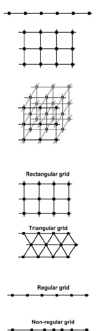
Depending on the dimension of the problem, the numerical grid can be one, two and
three dimensional (1D, 2D, 3D) (Fig. 7.1).
r
Depending on the shape of the basic elements, the grid can be rectangular and triangular
(Fig. 7.2).
r
Depending on the distribution of nodal points, the grid can be regular and non-regular
(irregular) (Fig. 7.3).
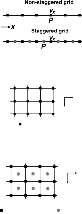
r
Depending on the distribution of different variables within the grid, it can be non-
staggered or staggered (Fig. 7.4).
83
84 Numerical solutions of the equations
1D grid
2D grid
3D grid
Fig. 7.1 Examples of 1D, 2D and 3D numerical grids.
Fig. 7.2 Examples of rectangular and triangular 2D numerical grids.
Fig. 7.3 Examples of regular and non-regular 1D numerical grids.
7.1 Grids 85
Fig. 7.4 Examples of non-staggered and staggered 1D numerical grids.
Non-staggered 2D grid
V
x
,
V
y
,
P,
,
y
rh
x
Fig. 7.5 Example of a non-staggered 2D numerical grid.
Half-staggered 2D grid
basic nodes
additional nodes
V
x
, V
y
, r, h
P
y
x
Fig. 7.6 Example of a half-staggered 2D numerical grid.
The simplest grids are non-staggered. All variables are defined at the same
nodal points (Fig. 7.5). When using finite differences (FD) with such a grid, all
equations are formulated at the same nodal points. Non-staggered grids are the
natural choice for solving the Poisson, heat conservation and advective transport
equations.
In the staggered grid, several types of nodal points exist (Fig. 7.6)atwhich
different variables are defined. A half-staggered grid in two dimensions (Fig. 7.6)
is a combination of a basic non-staggered grid, with an additional set of points
defined at the centres of cells formed by the basic grid. Part of the variables is then
defined at these additional nodes and not at the basic nodal points. A half-staggered
grid is convenient for solving the combination of Stokes and continuity equations
86 Numerical solutions of the equations
Fully staggered 2D grid
V
x
V
y
P
,
y
rh
x
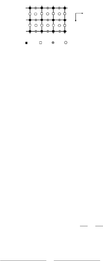
Fig. 7.7 Example of a fully staggered 2D numerical grid.
in case of constant viscosity when unknown parameters are components of velocity
(v
x
, v
y
) defined at the basic nodes, and pressure (P) defined at the additional nodes
(Fig. 7.6). Accordingly, x-andy-Stokes equations (Eq. 5.22) are formulated at
basic nodes, whilst the continuity equation is formulated at the additional nodes.
Yet, half-staggered grids are less natural for mechanical and thermomechanical
problems with variable viscosity.
Fully staggered grids are applied in two and three dimensions and consist of a
combination of several types of nodal points having different geometrical positions
(Fig. 7.7). Different variables are then defined at different nodal points. Differ-
ent equations are also formulated at different nodal points. Despite the apparent
geometrical complexity, fully staggered grids are the most convenient choice for
thermomechanical numerical problems with variable viscosity when finite dif-
ferences are used for solving the continuity, Stokes and temperature equations.
Discretisation of thermomechanical equations on the fully staggered grid is very
natural and gives simple FD formulas. Also, the accuracy of a numerical solution
obtained on a fully staggered grid is notably (up to four times, Fornberg, 1995)
higher then that on a non-staggered grid. Therefore: ‘think in a fully staggered
way!’ (I’ve done this since 2002).
7.2 Discretisation of the equations
The discretisation of the equations depends on the type of numerical grid that
is employed. The following discretisation schemes can for example be used to
describe the 2D incompressible continuity equation
∂v
x
∂x
+
∂v
y
∂y
= 0 in the case of
non-staggered (half-staggered) and a fully staggered 2D grid.
Non-staggered (half-staggered) grid (Fig. 7.8):
v
x3
− v
x1
+ v
x4
− v
x2
2x
+
v
y2
− v
y1
+ v
y4
− v
y3
2y
= 0. (7.1)