Gerya T. Introduction to Numerical Geodynamic Modelling

3.3 Geometrical and global indexing of unknowns 47

(e) The last equation in the ﬁnal system (diagonal matrix) will have the form

n−1

n,n

= R

n−1

, (3.15)

i.e., will only contain only one coefﬁcient L

n−1

n,n

for the unknown x

and right-hand side

n−1

. Then S

can be directly calculated as

n−1

n,n

. (3.16)

(f) The penultimate equation will have the form

n−2

n−1,n−1

n−1

+ L

n−2

n−1,n

= R

n−2

n−1

, (3.17)

and S

n−1

can be calculated with the already known S

as follows

n−1

n−2

n−1

− L

n−2

n−1,n

n−2

n−1,n−1

. (3.18)

(g) Repeat for all other unknowns from S

n−2

to S

The main advantage of direct methods is that the solution can be done to computer

accuracy and no iterations are needed. Among their disadvantages are (i) large

amounts of consumed memory, typically proportional to the square of the number

of unknowns and (ii) large amounts of operations, typically proportional to the

square or even to the cube of the number of unknowns. Due to limitations in

computer power, direct solvers are more often used in 1D and 2D modelling,

particularly for solving numerical problems, where iterative solvers are inefﬁcient.

3.3 Geometrical and global indexing of unknowns

In composing the system of Equations (3.4)–(3.7), we indexed our unknown param-

eters 

, 

and 

in 1D using the principle of growing index of the param-

eter with x-coordinate of the respective geometrical point to which this unknown

is assigned (cf. points 1, 2, 3 and 4 in Fig. 3.3). We may then have an impression

that a general system of equations (3.8) can only be applicable for 1D problems

since in 2D unknown parameters should have both horizontal and vertical indices,

for example 

i,j

and respectively S

i,j

. This is not correct and it is a small, but

important point to understand. Geometrical indexing of unknowns 

i,j

in a 2D

grid is different from overall global indexing of these unknowns given by S

and

used in the system of equations (3.8). Global indexing of unknowns (Fig. 3.4)is

always needed when direct methods are used for solving the equations as one has

to compose the matrix {L} and vector {R}. In the case of iterative solutions, one

can formulate equations (such as (3.4)–(3.7)) using a geometrical indexing.

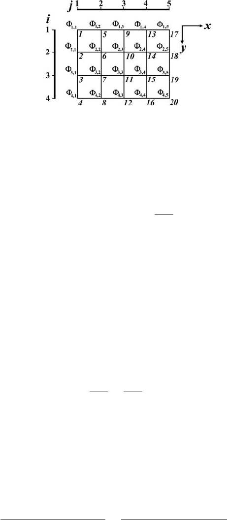
48 Numerical solutions of partial differential equations

Fig. 3.4 Geometrical indexing of gravity potential values 

i,j

assigned to the nodes

of 2D grid and global indexing (italic numbers) of these parameters in the vector

{S}. The global indexing is done by columns of nodal points.

Programming exercises and homework

Exercise 3.1

Solve the 1D Poisson equation, written in form

∂



∂x

= 1, on a regular grid of 1000

points with ﬁnite differences and visualise the solution. The model length is 1000

km. Use sparse initialisation for the matrix of coefﬁcients {L}, i.e. L =sparse(1000,

1000). Compose a matrix {L} and a right-hand side vector {R} (use Eqs. (3.4)–

(3.7) as an example) and obtain the solution vector {S} with a direct solver (in

MATLAB with the command S =L\R). Use  = 0 as the boundary condition for

the two external nodes of the grid (e.g. Fig. 3.3). An example is in Poisson1D.m.

Exercise 3.2

Solve the 2D Poisson equation with ﬁnite differences and visualise the solution.

The governing equation is given by

∂



∂x

∂



∂y

= 1, (3.19)

on a regular grid of 31 × 41 points. The model size is 1000 × 1500 km. Use

the principle of global indexing in 2D as shown in Fig. 3.4. A ﬁnite-difference

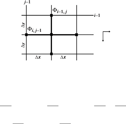
representation of the Poisson equation in 2D can be derived from Eq. (3.19)

by analogy with Eq. (3.2), but applied separately for the x and y directions

(Fig. 3.5)



i,j−1

− 2

i,j

+ 

i,j+1

x



i−1,j

− 2

i,j

+ 

i+1,j

y

= 1, (3.20)

Programming exercises and homework 49

i+1

j+1

i, j

i+1, j

i, j+1

Fig. 3.5 2D numerical grid stencil (5-point cross) used for formulating the Poisson

equation by using ﬁnite differences on a regular rectangular grid.

or by assembling coefﬁcients at each unknown



x





i,j−1



x





i,j+1



−2

x

−2

y





i,j



y





i−1,j



y





i+1,j

= 1. (3.21)

Use  = 0 as the boundary conditions for all external nodes of the grid. Compute

the global index of unknown k, based on geometrical indices i and j (Fig. 3.5)as

k = N

× (j − 1) + i, (3.22)

where N

is vertical resolution. An example is in Poisson2D_direct.m.

Exercise 3.3

Solve the same 2D problem using Gauss–Seidel iterations. Use Eq. (3.9) to compute

residuals. Use θ = 1.5 as a relaxation factor for all points (Eq. (3.10)). Plot

the gravitational potential and residuals every 10 iterations. An example is in

Poisson2D_Gauss_Seidel.m.

Exercise 3.4

Solve the same 2D problem using Jacobi iterations. Use θ =1.0 as relaxation factor

for all points (Eq. (3.10)). An example is in Poisson2D_ Jacobi.m.

Stress and strain

Theory: Deformation and stresses. Deﬁnition of stress, strain and

strain-rate tensors. Deviatoric stresses. Mean stress as a dynamic (non-

lithostatic) pressure. Symmetry of stress tensor. Stress and strain rate

invariants.

Exercises: Computing the strain rate tensor components in 2D from the

material velocity ﬁelds.

4.1 Stress

Tensors are ﬁeld variables which characterise the internal state of a continuum and

are, perhaps, the most difﬁcult quantities to intuitively understand. Indeed, at least

three of them have to be used in the following and these are the stress, strain and

strain rate tensors.

Stress is the internal distribution and intensity of force acting at any point

within a continuum in response to various internal and external loads applied

to the continuum. Stress is deﬁned as a force per unit area and we can easily

‘apprehend’ its effect by pressing two ﬁngers against each other – equal force is

applied from both sides and therefore nothing moves, but we have a feeling of

pressure between the ﬁngers, which is a sign of the presence of stress. This stress

is directly proportional to the applied force – the stronger we press the stronger

the feeling is. On the other hand, the stress is inversely proportional to the contact

surface between the ﬁngers – if we press one ﬁnger with the nail of the other the

feeling is much stronger because the same force is applied to a much smaller area.

This is why pricking a ﬁnger with a needle is so painful – the force applied to the

needle is not big but the contact surface of the needle with the ﬁnger is very small

and the resulting stress is consequently very big.

52 Stress and strain

(x)

-s

(b)(a)

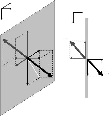
Fig. 4.1 Components of stress tensor deﬁned from the force balance on a surface.

(a) relationship between the stress components (thin arrows σ

, σ

and

−σ

, −σ

) and force vectors (thick arrows



(x)

and −



(x)

) acting on the

two sides of the unit element (grey) of a Lagrangian surface orthogonal to x-axis

(i.e. x-surface). White arrow in (a) shows the direction of shear along the surface.

(b) physical analogy: normal and shear stress components acting on a thin plate

(cross-section of the plate in x-y-plane is shown).

In order to characterise the stress tensor, let us consider the force



(x)

acting

on a unit element of a Lagrangian x-surface (i.e. surface orthogonal to the x-axis)

(Fig. 4.1(a)). First of all, we need to understand that the force vector



(x)

acting

on one side of the surface element is balanced by the counterforce vector −



(x)

which acts on the other side, and therefore this stressed surface element does

not move. Thus, in order to characterise the force balance state of the stressed

surface element, one needs to characterise the magnitude and direction of the force

(balanced by the counterforce) acting on this element. Let us adopt a convention

that the characterisation will be based on the force vector



(x)

, applied to the side

of the x-surface from which the x-axis is exiting. As we will see in the following,

according to this convention, extensional stresses are positive as is usually assumed

in continuum mechanics (e.g., Ranalli, 1995). Notice that this usual continuum

mechanics convention is opposite to that used in the book of Turcotte and Schubert

(2002), where stresses are taken positive under compression (which geoscientists

ﬁnd more intuitive since pressure is also positive under compression).

The force vector



(x)

can obviously be decomposed into three components (σ

, σ

) parallel to each coordinate axis (Fig. 4.1(a)). These are the components

4.1 Stress 53

of the stress tensor since force



(x)

is acting on the unit element. According to

the common continuum mechanics convention (e.g. Ranalli, 1995), which is again

opposite to that used in the book of Turcotte and Schubert (2002), the ﬁrst index

(i) of a stress component σ

denotes the axis along which this stress component

is taken (i.e. i =z for the component parallel to the z axis) and the second index

(j) indicates the surface on which force balance is considered (i.e. j =x for the

surface orthogonal to x axis). It should be pointed out that our ‘hard choice’ of a

stress deﬁnition and notation is, indeed, very convenient for formulating several

crucial equations, such as the momentum equation and the rheological constitu-

tive relationships, which is the main reason why we deviated from the ‘geological

convention’. On the other hand, our vertical axis y, is always pointing down, thus

preserving common ‘geological logic’ that the vertical coordinate is depth (and not

height as in continuum mechanics) and increases downward rather than upward.

A stress component that is orthogonal to the surface (cf. σ

in Fig. 4.1(a))is

called a normal stress component and the components which are parallel to the

surface are called shear stress components (cf. σ

and σ

in Fig. 4.1(a)). The

normal stress component characterises the magnitude of extension/compression

across the surface. The two shear stress components characterise the magnitude

and direction (cf. white arrow in Fig. 4.1) of shearing applied along the consid-

ered surface. A useful physical analogy (Fig. 4.1(b)) – if one imagines that the

force and counterforce are applied on two sides of a very thin plate, then the

normal component deﬁnes how strongly two opposite surfaces of the plate are

forced to be shifted from/toward each other and the shear stress components deﬁne

where and how strong these surfaces are forced to be shifted parallel to each

other.

In order to fully characterise the force balance at a point (a small material

volume), it is convenient to represent the stress tensor as a N × N matrix where N

is the dimension of the problem such that in one, two and three dimensions we will

have one, four and nine stress components respectively (Fig. 4.2)

1D stress tensor, N = 1 (Fig. 4.2(a)): σ

(

)

2D stress tensor, N = 2 (Fig. 4.2(b)): σ





3D stress tensor, N = 3 (Fig. 4.2(c)): σ









where i and j are symbolic coordinate indices (x, y, z) which vary in vertical and

horizontal directions, respectively. In continuum mechanics books a numerical

54 Stress and strain

-s

1D 3D

(a)

(b) (c)

Fig. 4.2 Components of the stress tensor (black and grey arrows) deﬁned in one-

(a) two- (b) and three- (c) dimensions on faces of a small interval, square and cube,

respectively. The faces are always oriented orthogonal to the main axis. Thin lines

in (b) and (c) connect pairs of shear stress components which should be equal to

each other in the absence of internal sources of angular momentum.

(1, 2, 3) notation for the coordinate indices i and j and stresses (σ

, σ

,etc.)

is commonly used as well (e.g. Ranalli, 1995). Note that i and j are indices and not

spatial coordinates of geometric points.

Normal stresses are always located on the main diagonal of the matrix. Due

to the condition of force balance in the absence of internal sources of angular

momentum, this matrix is symmetric relative to the main diagonal so that

= σ

i.e. (Fig. 4.2(b), (c))

= σ

Like components of a vector, components of the stress tensor at a point depend on

the orientation of the coordinate system. We will discuss this in more detail later

in relation to elasticity (Chapter 12).

In continuum mechanics, pressure is deﬁned as the mean normal stress:

P =−(σ

+ σ

)/3 (4.1)

where the negative sign on the right-hand side of Eq. (4.1) reﬂects another con-

vention according to which pressure is positive under compression. Pressure is an

4.1 Stress 55

invariant and, thus, does not change with changing the coordinate system.Inthe

case of a hydrostatic stress state (which is the state of a ﬂuid at rest) all shear

stresses are zero and all normal stresses are equal to each other

= σ

= 0 (4.2a)

= σ

=−P. (4.2b)

In geosciences, pressure is often considered as corresponding to the hydrostatic

condition everywhere and it is computed as a function of depth y and vertical

density proﬁle ρ(y)

P (y) = P

+ g



ρ(y)dy, (4.3)

where P

= 0.1 MPa is pressure on the Earth’s surface and g is the gravitational

acceleration.

This simpliﬁcation does not hold when deformations of geological media occur

and real dynamic pressure may notably deviate from the lithostatic value given by

Eq. (4.3).

It is often convenient to deﬁne the deviatoric stresses σ



, which are deviations

of stresses from the hydrostatic stress state (i.e., deviations from conditions (4.2))



= σ

+ Pδ

, (4.4)

where δ

is the Kronecker delta: δ

= 1wheni =j and δ

= 0wheni = j, i and

j are coordinate indices (x, y, z). The Kronecker delta is a peculiar abbreviation

used in the mechanics of continuum. It only takes values of either 1 or 0 and is

analogous to the logical operator ‘if’ used in many programming languages. Any

equation with δ

represents a group of equations. For example, Eq. (4.4)in3D

represents the following equations:

Normal deviatoric stresses



= σ

+ P,



= σ

+ P,



= σ

+ P,

and shear stresses which are entirely deviatoric



= σ



= σ



= σ



= σ



= σ



= σ

56 Stress and strain

It is worth mentioning that the sum of the normal deviatoric stresses is zero by

deﬁnition (Eq. (4.4))



+ σ



+ σ



= 0,

since

+ σ

=−3P.

The second invariant of the deviatoric stress tensor can be calculated as follows:





, (4.5)

where the indices ij imply a summation! This is another abbreviation that is com-

monly used in continuum mechanics and makes equations shorter (but, indeed, not

easier to understand for inexperienced readers). The spelled-out form of Eq. (4.5)

is much longer





2

+ σ

2

+ σ

2

+ σ



, (4.6a)

or, using the condition of force balance σ

=σ





2

+ σ

2

+ σ

2



+ σ

. (4.6b)

The second stress invariant σ

does not depend on the coordinate system and

characterises the local deviation of stresses in the medium from the hydrostatic

state.

4.2 Strain and strain rate

Another important quantity is the strain γ , that characterises the amount of defor-

mation. Strain is dimensionless and is computed as the ratio of displacement L

to the initial length of deforming body L (Fig. 4.3)

γ =

L

. (4.7)

By analogy with stress, one can discriminate normal and shear strain corresponding

to axial and shear deformation, respectively (Fig. 4.3(a) and (b)).

The deﬁnition of strain given by Eq. (4.7) can only be applied in cases of rela-

tively simple axial and shear deformations. In case of more complex deformation,

the strain tensor ε

,isdeﬁnedas



∂u

∂x

∂u

∂x



, (4.8)

Gerya T. Introduction to Numerical Geodynamic Modelling

Подождите немного. Документ загружается.