Genshiro Kitagawa. Introduction to Time Series Modeling (Введение в моделирование временных рядов)

Подождите немного. Документ загружается.

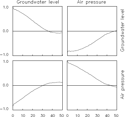
CROSS-COVARIANCE FUNCTION 29

Figure 2.6 Autocorrelati on functions and cross-correlation functions of the

groundwater level and barometric pressure data.

Example (Grandwater level data) Figure 2.6 shows the cross-

correlation function between the groundwater level data and the baro-

metric pressur e data illustrated in Figure 1.1(h). A very strong correla-

tion between the two variables is seen.

Problems

1. Show that a weakly stationar y Gaussian time series is stro ngly sta-

tionary.

2. Is a strongly stationary time series wea kly stationary?

3. Show that the autocovariance func tion of a statio nary time series is an

even function.

4. Obtain the autocovariance fu nction of a time series that satisﬁes y

−cv

n−1

, where |c| < 1 and v

is a white noise with mean 0 and

variance 1.

5. Assuming that C

,.. ., is the au tocovariance function of a station-

30 THE COVARIANCE FUNCTION

ary time series, show that the matrix

C =







··· C

k−1

··· C







is positive semi-deﬁnite.

6.(1) What is the expected value of the sample autocovariance fu nction

(2) Discuss the r e ason that the sum is divided by N, no t by N −k, in

the deﬁnition of the sample autocovariance f unction.

7.(1) Assuming that the time ser ies is a Gaussian wh ite noise, obtain th e

distributions of

and

(2) Using the results of (1), consider a method for checking whether

or not a time series is white.

Chapter 3

The Power Spect rum and the

Periodogram

In this section, the spectral analysis method is introduced as a basic tool

for stationary time series analysis. By means of spectral analysis, we

can capture the characteristics of time series by decomposin g time se-

ries into trigonometric f unctions at each frequency a nd by representing

the features with the strength of ea ch periodic component. The subjects

discussed here will lead to the deﬁnition of the power spectr um and the

periodogram of time series, computational methods, variance redu ction

and smoothing methods. Moreover, an efﬁcient method of computing pe-

riodograms is presented using fast Fourier transforms (FFT). The readers

interested in the spectral analysis of time series are referred to Brillinger

(1974), Bloomﬁed (1976), Ak a ike and Nakagawa (1989) and Brockwell

and Davis (1991).

3.1 The Power Spectr um

If the autocovariance function C

rapidly dec reases as the lag k increases

and satisﬁes

∞

∑

k=−∞

| < ∞,

we can deﬁne the Fourier transform of C

The function de ﬁned o n the freque ncy −1/2 ≤ f ≤ 1/2,

p( f ) =

∞

∑

k=−∞

−2

ik f

, (3. 1)

is called the power spe ctral density function or simply the po wer spec-

trum.

Since the auto c ovariance function is an even function and satisﬁes

= C

−k

, the power spectrum can also be expressed as

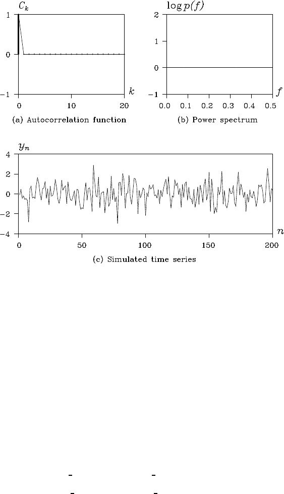
32 THE POWER SPECTRUM AND THE PERIODOGRAM

Figure 3.1 Autocorrelation function, power spectrum, and realization of a white

noise with variance

= 1.

p( f ) =

∞

∑

k=−∞

cos(2

k f ) −i

∞

∑

k=−∞

sin(2

k f )

∞

∑

k=−∞

cos2

k f = C

+ 2

∞

∑

k=1

cos2

k f . (3.2)

The power spec trum represents a time series in terms of trigonomet-

ric functions with various freq uencies an d expr e sses the characteristics

of a time series by the magnitudes of these cyclic components. On the

other hand, if a power spectrum is given, then the autocovariance func-

tion can be obta ined via the inverse Fourier transform

−

p( f )e

ik f

df =

−

p( f )cos 2

k f df . (3.3)

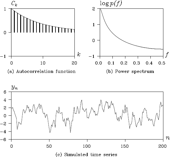
THE POWER SPECTRUM 33

Figure 3.2 Autocorrelation function, power spectrum, and realization of a ﬁrst-

order AR model with a = 0.9.

Example (The power spectrum of white noise) The a utocovariance

function of a white noise is given by C

and C

= 0 for k 6= 0.

Therefore, the power sp ectrum of a white noise becomes

p( f ) =

∞

∑

k=−∞

cos2

k f = C

, (3.4)

taking a constant value for any frequency f . It means that a white noise

contains cyclic compo nents of various frequencies with the same mag-

nitude. Plots ( a), (b) and (c) in Figure 3.1 show the autocorr e la tion func-

tion and the power spectrum of a white no ise with variance

= 1 and

realizations of white noise genera te d by the simulation. The simulation

method for a time series from an assumed model will be introduced later

in Chapter 16.

Example (Power spectrum of an AR model) Assume that w

is a

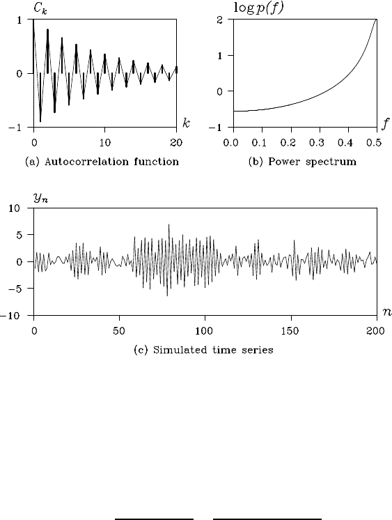
34 THE POWER SPECTRUM AND THE PERIODOGRAM

Figure 3.3 Autocorrelation function, power spectrum, and realization of a ﬁrst-

order AR model with a = −0.9.

white noise with variance

. If a time series is generated by a ﬁrst-

order autoregressive mod el y

= ay

n−1

, the autocovariance fu nction

is given by C

(1 −a

)

−1

|k|

and then the power spe ctrum of th is

time series can be evaluated as

p( f ) =

|1 −ae

−2

i f

1 −2a cos2

f + a

. (3.5)

Plots (a), (b) and (c) of Figure 3.2 show the autocorrelation func-

tion, the power spectrum and the re alization, which were generated by

the simulation for a ﬁrst autoregressive model with a = 0.9. Similarly,

Figure 3.3 shows the case of a ﬁrst-order autoregressive model with a

negative coefﬁcient a = −0.9. The autocorrelation f unction is very wig-

gly, and unlike the case of positive c oefﬁcient, the power spectrum is an

increasing function of the frequency f .

If a time series follows a second-order AR model y

= a

n−1

THE POWER SPECTRUM 35

Figure 3.4 Autocorrelation function, power spectrum, and realization of a

second-order AR model with a

= 0.9

√

3 and a

= −0.81.

n−2

+ w

, the auto c orrelation function satisﬁes

1 −a

, R

= a

k−1

+ a

k−2

, (3.6)

and the power spectrum can be evaluated as

p( f ) =

|1 −a

−2

i f

−a

−4

i f

1 −2a

(1 −a

)cos 2

f −2a

cos4

f + a

+ a

. (3.7)

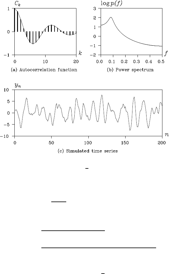
Figure 3.4 shows (a) the autocorrelation function, (b) the power spec-

trum and (c) a realization, which were generated by the simulation for

a second-order AR model with a

= 0.9

√

3 and a

= −0.81. The auto-

correlation function is oscillatory, and the power spec trum has a peak

around at f = 0.1.

36 THE POWER SPECTRUM AND THE PERIODOGRAM

3.2 The Periodogram

Given a time series y

,···, y

, the periodogram is deﬁned by

N−1

∑

k=−N+1

−2

ik f

+ 2

N−1

∑

k=1

cos2

k f

, (3.8)

where the sample autocovariance function

is substituted for the auto-

covariance function C

of equations (3.1) and (3.2).

In the deﬁnition of the periodogram, we consider only the natural

frequencies deﬁned by f

= j/N, j = 0,···,[N/2]. Here [N/2] denotes

the maximum integer, which do es not exceed N/2. An extension of the

periodogram

ˆp( f ) =

N−1

∑

k=−N+1

−2

ik f

, −0.5 ≤ f ≤ 0.5, (3.9)

obtained by extending the domain to the continuous interval [0,1/2] is

called the sample spectrum.

In other words, the periodogram is obtained from the sample spec-

trum by restricting its domain to the natur a l frequencies. Corresponding

to the relations of (3.3), the following relation holds between the sample

spectrum and the sample autocovariance function,

−

ˆp( f )e

ik f

df , k = 0,···, N −1. (3.10)

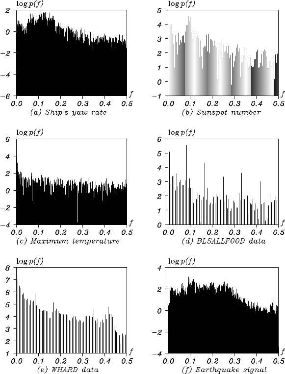
Example (Periodograms) Figure 3.5 shows the periodograms of the

univariate tim e serie s corresponding to Fig ures 1.1 (a)–(f). Note that the

vertical axis here has a logarithmic scale.

Plot (a) shows the periodogram of the ship’s yaw rate. A fairly strong

periodic component with an approximate 10-second period, i.e., f = 0.1,

is observed.

Plot (b) shows the periodogram of the annual sunspot numbe r ser ie s.

A strong periodic c omponen t with an app roximate 1 0-year period ( f =

0.1) is shown. However, because of the strong variation, oth er periodic

components canno t be clearly seen.

In the periodogram of the maximum temperature data shown in plot

(c), there is no apparent periodicity.

In the periodogram of the BLSALLFOOD data shown in plot (d),

a sharp peak is seen at the frequency f = 1/12 corr esponding to the

THE PERIODOGRAM 37

Figure 3.5: Periodograms of the data of Figure 1.1 (on a logarithmic scale).

38 THE POWER SPECTRUM AND THE PERIODOGRAM

seasonal components. The fr e quencies o f the other four peaks are integer

multiples of the frequency of the main peak and are c onsidered to be the

higher harmonics of the nonlinear waveform.

Similar peaks can be seen in the WHARD d a ta shown in plot (e), but

they ar e not as signiﬁcant as the ones shown in plot (d).

The pe riodogram of seismic wave data of plot (f) shows two plateau s

around f = 0.1 and f = 0.25, a nd sharp peaks are seen at f = 0.07 and

f = 0.1.

We note the pro perties of the periodogram hereafter. The peri-

odogram and the sample spectrum are asymptotically unbiased and sat-

isfy

lim

N→∞

E{ ˆp( f )} = p( f ) =

∞

∑

k=−∞

cos2

k f . (3.11)

This means that at each freq uency f , the expectation of the sample spec-

trum converges to the true spectrum as the number of data points in-

creases. However, it does not imply the consistency of ˆp( f ), that is, the

sample spectrum ˆp( f ) does not necessarily converge to p( f ) as the num-

ber of data points incre a ses. Actu a lly,

2 ˆp( f

)

p( f

)

,···,

2 ˆp( f

[

]−1

)

p( f

[

]−1

)

, (3.12)

indepen dently follow the

distribution with two degrees of freedom,

and ˆp(0)/p(0) and ˆp(0.5)/p(0.5) follow the

distribution with one

degree of f reedom. Therefore, the variance of the periodo gram is con-

stant, independent of the sample size N. Thus the periodogram cannot

be a con sistent estimator.

Example (Sample autocorrelation functions and periodograms)

Figures 3.6 (a) and (b) show the sample autocorrelation function an d

the p e riodogram, respec tively, of the realizations of white noise with a

sample size N = 200, which are generated similarly to Figure 3.1(c).

Sample autocorrelations are close to zero and are almost contained in

the c onﬁdence in te rval [−200

−1/2

,200

−1/2

] ≃ [−0.07,0.07]. The theo -

retical spectrum of the white noise is a constant, log p( f ) ≡0 in this case.

However, the periodogr am ﬂu c tuates sharply, indic a ting that it cannot be

a good estimate of th e spectrum.

Figures 3.6 (c)–(f ) show the sample autocorrelation functions and

the periodogram of realizations of white noise with sample sizes 800 and

3200. The sample autocorrelations

converge to the true value C

as the