Fowler A. Mathematical Geoscience

Подождите немного. Документ загружается.

Chapter 1

Mathematical Modelling

This book concerns the application of mathematics to problems in the physical sci-

ences, and particularly to problems which arise in the study of the environment.

Much of the environment consists of ﬂuid—the atmosphere, the ocean—and even

those parts which are solid may deform in a ﬂuid-like way—ice sheets, glaciers,

the Earth’s mantle; as a consequence, one way into the study of the environment

is through the study of ﬂuid dynamics, although we shall not follow that approach

here. Rather, we shall approach the study of environmental problems as applied

mathematicians, where the emphasis is on building a suitable mathematical model

and solving it, and in this introductory chapter, we set out the stall of techniques and

attitudes on which the subsequent chapters are based.

There are two particular points of view which we can bring to bear on the math-

ematical models which describe the phenomena which concern us: these are the

dynamical systems approach, or equivalently the bifurcation theory approach; and

the perturbation theory approach. Each has its place in different contexts, and some-

times they overlap.

The bifurcation theory approach is most usually (but not always) brought to bear

on problems which have some kind of (perhaps complicated) time-dependent be-

haviour. The idea is that we seek to understand the observations through the under-

standing of a number of simpler problems, which arise successively through bifur-

cations in the mathematical model, as some critical parameter is changed. A classic

example of this approach is in the study of the origin of chaos in the Lorenz equa-

tions, or the onset of complicated forms of thermal convection in ﬂuids.

In its simplest form (e.g., in weakly nonlinear stability theory) the perturbative

approach is similar in method to the bifurcational one; however, the ethos is rather

different. Rather than try and approach the desired solution behaviour through a

sequence of simpler behaviours, we try and break down the solution by making

approximations, which (with luck) are in fact realistic. In real problems, such ap-

proximations are readily available, and part of the art of the applied mathematician

is having the facility of being able to judge how to make the right approximations.

In this book, we follow the perturbative approach. It has the disadvantage of be-

ing harder, but it is able to get closer to a description of how realistic systems may

actually behave.

A. Fowler, Mathematical Geoscience, Interdisciplinary Applied Mathematics 36,

DOI 10.1007/978-0-85729-721-1_1, © Springer-Verlag London Limited 2011

2 1 Mathematical Modelling

1.1 Conservation Laws and Constitutive Laws

The basic building blocks of continuous mathematical models are conservation

laws. The continuum assumption adopts the view that the physical medium of con-

cern may be considered continuous, whether it be a porous medium (for exam-

ple, sand on a beach) or a ﬂuid ﬂow. The continuum hypothesis works whenever

the length or time scales of interest are (much) larger than the corresponding mi-

croscale. For example, the formation of dunes in a desert (length scale hundreds of

metres) can be modelled as a continuous process, since the microscale (sand grain

size) is much smaller than the macroscale (dune length). Equally, the modelling of

large animal populations or of snow avalanches treats the corresponding media as

continuous.

Conservation laws arise as mathematical equations which represent the idea that

certain quantities are conserved—for example, mass, momentum (via Newton’s

law) and energy. More generally, a conservation law refers to an equation which

relates the increase or decrease of a quantity to terms representing supply or de-

struction.

In a continuous medium, the typical form of a conservation law is as follows:

∂φ

∂t

+∇.f =S. (1.1)

In this equation, φ is the quantity being ‘conserved’ (expressed as amount per unit

volume of medium, i.e., as a density; f is the ‘ﬂux’, representing transport of φ

within the medium, and S represents source (S > 0) or sink (S < 0) terms. Deriva-

tion of the point form (1.1) follows from the integral statement



φdV =−



∂V

f.ndS +



SdV, (1.2)

after application of the divergence theorem (which requires f to be continuously

differentiable), and by then equating integrands, on the basis that they are continuous

and V is arbitrary. Derivation of (1.1) thus requires φ and f to be continuously

differentiable, and S to be continuous.

Two basic types of transport are advection (the medium moves at velocity u,so

there is an advective ﬂux φu) and diffusion, or other gradient-driven transport (such

as chemotaxis). One can thus write

f =φu +J, (1.3)

where J might represent diffusive transport, for example.

Invariably, conservation laws contain more terms than equations. Here, for ex-

ample, we have one scalar equation for φ, but other quantities J and S are present

as well, and equations for these must be provided. Typically, these take the form of

constitutive laws, and are usually based on experimental measurement. For example,

diffusive transport is represented by the assumption

J =−D∇φ, (1.4)

1.2 Non-dimensionalisation 3

where D is a diffusion coefﬁcient. In the heat equation, this is known as Fourier’s

law, and the heat equation itself takes the familiar form

∂

∂t

(ρc

T)+∇.(ρc

T u) =∇.(k∇T)+Q, (1.5)

where Q represents any internal heat source or sink.

1.2 Non-dimensionalisation

Putting a mathematical model into non-dimensional form is fundamental. It allows

us to identify the relative size of terms through the presence of dimensionless pa-

rameters. Although technically trivial, there is a certain art to the process of non-

dimensionalisation, and the associated concept of scaling. We illustrate some of the

precepts by consideration of the heat equation, (1.5). We write it in the form (as-

suming density ρ and speciﬁc heat c

are constant)

∂T

∂t

+u.∇T = κ∇

T +H, (1.6)

where H = Q/ρc

. We have taken ∇.u =0, which follows from the conservation

of mass equation

∂ρ

∂t

+∇.(ρu) =0, (1.7)

together with the supposition of incompressibility in the form ρ = constant.

Suppose we are to solve (1.6) in a domain D of linear magnitude l, on the bound-

ary of which we prescribe

T =T

on ∂D, (1.8)

where T

is constant. We also have an initial condition

T =T

(x) in D, t =0, (1.9)

and we suppose u is given, of order U .

We can make the variables dimensionless in the following way:

x =lx

∗

, u =Uu

∗

,t=t

∗

,T=T

+(T )T

∗

. (1.10)

We do this in order that both dependent and independent dimensionless variables be

of numerical order one, written O(1). If we can do this, then we might suppose a

priori that derivatives such as ∇

∗

(∇ =l

−1

∇

∗

) will also be of numerical O(1),

and the size of various terms will be reﬂected in certain dimensionless parameters

which occur.

In writing (1.10), it is clear that l is a suitable length scale, as it is the size of D.

For example, if D was a sphere we might take l as its radius or diameter. We also

4 1 Mathematical Modelling

suppose that the origin is in D; if not, we could write x =x

+lx

∗

, where x

∈D:

evidently x

∗

=O(1) in D.

A similar motivation underlies the choice of an ‘origin shift’ for T . In the absence

of a heat source, the temperature will tend to the uniform state T ≡T

as t →∞.

If H =0, the ﬁnal state will be raised above T

(if H>0) by an amount dependent

on H .WetakeT to represent this amount, but we do not know what it is in

advance—we will choose it by scaling. The subtraction of T

from T before non-

dimensionalisation is because the model for T contains only derivatives of T ,so

that it is really the variation of T about T

whichwewishtoscale.

In a similar way, the time scale t

is not prescribed in advance, and we will choose

it also by scaling, in due course.

With the substitutions in (1.10), the heat equation (1.6) can be written in the form



κt



∂T

∗

∂t

∗





∗

.∇

∗

=∇

∗2

∗



κT



. (1.11)

This equation is dimensionless, and the bracketed parameters are dimensionless.

They are somewhat arbitrary, since t

and T have not yet been chosen: we now do

so by scaling.

The solution of the equation can depend only on the dimensionless parameters.

It is thus convenient to choose t

and T so that two of these are set to some

convenient value. There is no unique way to do this.

The temperature scale T appears only in the source term. Since it is this which

determines the temperature rise, it is natural to choose

T =

. (1.12)

It is also customary to choose the time scale so that the two terms of the advective

derivative on the left of (1.11) are the same size, and this gives the convective time

scale

. (1.13)

It is ﬁnally also customary (if sometimes confusing) to remove the asterisks (or

whatever equivalent symbol is used). If this is done, the dimensionless equation

takes the form



∂T

∂t

+u.∇T



=∇

T +1, (1.14)

where the Péclet number is

Pe =

, (1.15)

and the solution of the model depends only on this parameter (as well as the initial

condition). The boundary condition is

T =0on∂D, (1.16)

1.2 Non-dimensionalisation 5

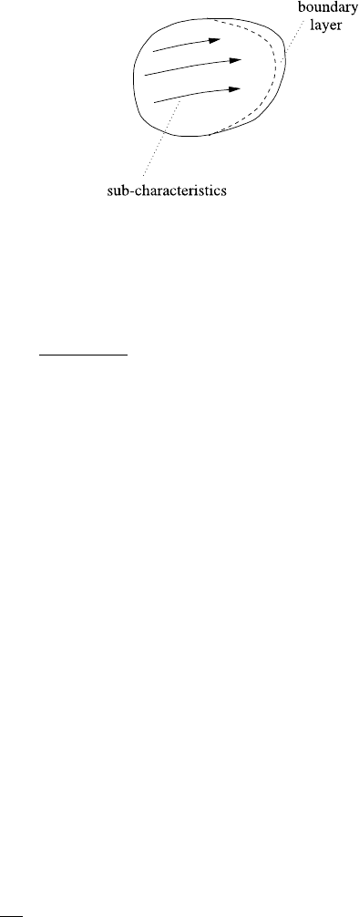
Fig. 1.1 Sub-characteristics

and boundary layer for

Eq. (1.14)whenPe 1. The

sub-characteristics are the

ﬂow lines dx/dt =u,andthe

boundary layer (of thickness

O(1/Pe)) is on the part of the

boundary where the ﬂow lines

terminate

and the initial condition is

T =θ(x) at t =0, (1.17)

where

θ(x) =

(lx) −T

T

. (1.18)

1.2.1 Scaling

A well-scaled problem generally refers to a model in which the dimensionless pa-

rameters are O(1) or less. Evidently, this can be ensured simply by dividing through

by the largest parameter in any equation. More importantly, if parameters are numer-

ically small, then (as we discuss below) approximate solutions can be obtained by

neglecting them. The problem is well-scaled if the resulting approximation makes

sense. For example, (1.14) is well-scaled for any value of Pe. However, the problem

εT

=ε∇

T +1, with ε 1, is not well scaled. One makes a problem well-scaled in

this situation by rescaling the variables, and we will see examples in our subsequent

discussion.

1.2.2 Approximations

Let us consider (1.14) with (1.16) and (1.17), and suppose that θ ≤O(1).IfPe 1,

we obtain an approximation by putting Pe =0: ∇

T +1 ≈0. Evidently, we cannot

satisfy the initial condition, and this suggests that we rescale t: put t =Pe τ , so that

(approximately)

∂T

∂τ

=∇

T +1; (1.19)

now we can satisfy the initial condition (at τ = 0) too. Often one abbreviates the

rescaling by simply saying, ‘rescale t ∼Pe, so that T

≈∇

T +1’.

6 1 Mathematical Modelling

On the other hand, if Pe  1, then T

+ u.∇T ≈0, and we can satisfy the ini-

tial condition; but we cannot satisfy the boundary condition on the whole of the

boundary ∂D, since the approximating equation is hyperbolic (its characteristics

are called ‘sub-characteristics’). To remedy this, one has to rescale x near the part of

the boundary where the boundary condition cannot be satisﬁed, and this is where the

sub-characteristics terminate. This gives a spatially thin region, called (evidently) a

boundary layer, of thickness 1/Pe (see Fig. 1.1).

Another case to consider is if θ  1, say θ ∼ Λ  1. We discuss only the

case Pe  1 (see also Question 1.6). Since T ∼ Λ initially, we need to rescale T ,

say T = Λ

T . Then Pe[

+u.∇

T ]=∇

T +

, and with

T = O(1),wehave

+u.∇

T ≈0forPe  1. The initial function is simply advected along the ﬂow

lines (sub-characteristics), and the boundary condition

T =0 is advected across D.

InatimeofO(1), the initial condition is ‘washed out’ of the domain. Following this,

we revert to T , thus T

+u.∇T =

(∇

T +1). Evidently T will remain ≈0inmost

of D, and in fact T ∼O(

). Putting T =

, χ satisﬁes χ

+u.∇χ =

∇

χ +1,

and there is a boundary layer near the boundary as shown in Fig. 1.1.Ifn is the

coordinate normal to ∂D in this layer, then n ∼

in the boundary layer. The ﬁnal

steady state has T ∼

, and this applies also for θ

∼

O(1).

These ideas of perturbation methods are very powerful, but a full exposition is

beyond the scope of this book. Nevertheless, they will relentlessly inform our dis-

cussion. While it is possible to use formal perturbation expansions, it is sufﬁcient in

many cases to give more heuristic forms of argument, and this will typically be the

style we choose.

1.3 Qualitative Methods for Differential Equations

The language of the description of continuous processes is the language of differ-

ential equations, and these will form the instrument of our discussion. The simplest

differential equation is the ordinary differential equation, and the simplest ordinary

differential equation (or ODE) is the ﬁrst order autonomous equation

˙x =f(x), (1.20)

where the notation ˙x ≡

indicates the ﬁrst derivative, and the use of an overdot

is normally associated with the use of time t as the independent variable, i.e., ˙x =

dx/dt.

The solution of (1.20) with initial condition x(t

) = x

can be written as the

quadrature

t =t



dξ

f(ξ)

, (1.21)

and, depending on the function f , this may be inverted to ﬁnd x explicitly. So, for

example, the solution of ˙x =1 −x

is x =tanh(t +c) (if |x(t

)|< 1).

1.3 Qualitative Methods for Differential Equations 7

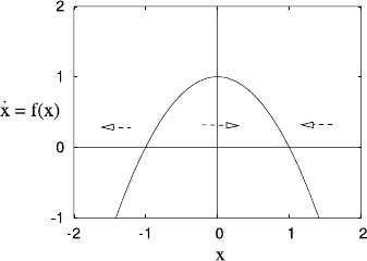
Fig. 1.2 The evolution of the

solutions of ˙x =f(x)(here

f = 1 −x

) depends only on

the sign of x

Going on with this latter example, we see that x →1ast →∞(and x →−1

as t →−∞), and in practice, this may be all we want to know. If a population

is subject to constant immigration and removal by mutual pair destruction, so that

˙x =1 −x

, then after a transient (a period of time dependence), the population will

equilibrate stably to x =1. But to ascertain this, all we need to know is the shape of

the curve f(x)=1 −x

. Simply by ﬁnding the zeros of 1 −x

and the slope of the

graph there, we can immediately infer that for all initial values x(0)>−1, x →1

as t →∞, while if x(0)<−1, then x →−∞as t →−∞: see Fig. 1.2. And this

can be done for any function f(x)in the equation ˙x =f(x).

This simple example carries an important message. Approximate or qualitative

methods may be just as useful, or more useful, than the ability to obtain exact results.

An extension of this insight suggests that it may often be the case that approximate

analytic insights can provide more information than precise, computational results.

1.3.1 Oscillations

If we move from ﬁrst order systems to second order systems of the form

˙x =f(x,y),

˙y =g(x,y),

(1.22)

more interesting phenomena can occur. This is the subject of phase plane analysis,

and the fundamental distinction between ﬁrst and second order systems is that peri-

odic oscillations can occur. An illuminating example is illustrated in Fig. 1.3, and is

typiﬁed by (but is not restricted to) the equations

˙x =y −g(x),

˙y =h(x) −y,

(1.23)

where the functions g and h are as shown in the ﬁgure: g is unimodal (e.g., like

g =xe

−x

) and h is monotonic decreasing (e.g., like h =1/(x −c)). The graphs of

g(x) and h(x) (and more generally, the curves where ˙x = 0 and ˙y =0) are called

the nullclines of x and y, and it is simple to see that where they intersect, there is

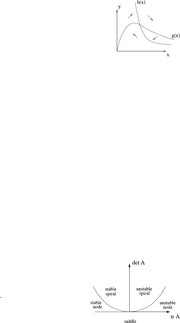
8 1 Mathematical Modelling

Fig. 1.3 Nullclines for (1.23)

a steady state solution, and also that in the four regions separated by the nullclines,

the trajectories wind round the ﬁxed point in a clockwise manner.

The next issue is whether the ﬁxed point is unstable. If we denote it as (x

∗

write x =x

∗

+X, y =y

∗

+Y , and linearise for small X and Y , then

U ≈



−g



−1



U, (1.24)

where U =





, and the derivatives are evaluated at the ﬁxed point. The stability

of such a two by two system with community matrix A =



−g



−1



is governed

by the trace and determinant of A. Solutions of (1.24) proportional to e

σt

exist if

−σ tr A +detA =0, and this delineates the stability regions in the (tr A, det A)

space as indicated in Fig. 1.4. In the present case, tr A =−g



−1, det A =g



−h



so that for the situation shown in Fig. 1.3, where h



< 0, det A>0, and the

ﬁxed point is an unstable spiral (or node) if g



< −1. When g



=−1, there is a Hopf

bifurcation, and if the system has bounded trajectories (as is normal for a model of

a physical process) then one expects a stable periodic solution to exist. Figure 1.5

illustrates a possible example.

1.3.2 Relaxation Oscillations

It is a general precept of the applied mathematician that there are three kinds of

numbers: small, large, and of order one. And the chances of a number being O(1)

Fig. 1.4 Characterisation of

ﬁxed point stability in terms

of trace and determinant of

the community matrix A.The

curve separating spirals from

nodes is given by

detA =

(trA)

1.3 Qualitative Methods for Differential Equations 9

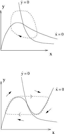
Fig. 1.5 Typical form of the

limit cycle for a system with

nullclines as in Fig. 1.3

Fig. 1.6 Typical form of

relaxation oscillation in phase

plane for (1.25)

are not great. Thus for systems of the form (1.22), it is often the case in practice

that the time scales for each equation are different, so that in suitable dimensionless

units, the second order system (1.23) might take the form

ε ˙x =y −g(x),

˙y =h(x) −y,

(1.25)

where the parameter ε is small. Now suppose that the nullclines y = g(x) and

y = h(x) for the system (1.25)areasshowninFig.1.6, i.e., g has a cubic shape.

Trajectories rotate clockwise, and linearisation about the ﬁxed point yields a com-

munity matrix A with trA =−(g



/ε) −1, det A =(g



−h



)/ε, thus with g



,the

ﬁxed point is a spiral or node, and with ε  1, trA ≈−g



/ε > 0, so it is unstable.

Thus we expect a limit cycle, and because ε 1, this takes the form of a relaxation

oscillation in which the trajectory jumps rapidly backwards and forwards between

branches of the x nullcline. For ε  1, x rapidly jumps to its quasi-equilibrium

y ≈ g(x), and then y migrates slowly ( ˙x ≈[h(x) −g(x)]/g



(x)) until g



= 0 and

x jumps rapidly to the other branch of g. Figure 1.7 showsthetimeseriesofthe

resulting oscillation. The motion is called ‘relaxational’ because the fast variable x

‘relaxes’ rapidly to a quasi-stationary state after each transient excursion.