Fowler A. Mathematical Geoscience

Подождите немного. Документ загружается.

40 1 Mathematical Modelling

where ˙c

≡∂c

/∂s. Substituting this into (1.180) and equating powers of τ , we ﬁnd

(s), (1.183)

where C

is arbitrary, and





−

1 +

−



. (1.184)

The arbitrary function C

arises because the order of the approximate equation is

reduced. In order to specify it, and other arbitrary functions of s which arise at each

order, we require that the solutions c

be smooth, and this requires that there be no

term on the right hand side of (1.184) proportional to 1/z as z → 0, in order that

logarithmic singularities not be introduced. Speciﬁcally, we require at each stage of

the approximation that

∂c

∂z



z +a

+···



; (1.185)

so that z

is smooth. Applying this to (1.184) requires that

(1 −C

), (1.186)

so that C

→1ass →∞, and then

=−

(s) +C



1 +



. (1.187)

At O(1/τ

), we then have



+4zc

1zz



−(˙c

−c

) +





−

)

1 +



1 +





, (1.188)

and applying the regularity condition (1.185), we ﬁnd, after some algebra,

=2(1 −C

, (1.189)

so that C

→C

s as s →∞. Thus, ﬁnally we obtain the local similarity solu-

tion

u ≈−ln





−t +

c(x −x

)

4[−ln(t

−t)]



, (1.190)

where c ≈C

(s), s = ln τ =ln[−ln(t

−t)].

1.4 Qualitative Methods for Partial Differential Equations 41

1.4.9 Reaction–Diffusion Equations

The development of mathematical biology in the last thirty years has led to one

particular pedagogical example of wave and pattern formation, and that is in the

coupled sets of equations known as reaction–diffusion equations. The general type

∂u

∂t

(u) +∇.[D

∇u

], (1.191)

for n reactants u

,...,u

, where the summation convention (sum over repeated

sufﬁxes, here j) is implied, but much of what is known about the behaviour of such

systems can be illustrated with the two-species equations

=f(u,v)+D

∇

=g(u,v) +D

∇

(1.192)

The phenomena which we ﬁnd are closely allied to the behaviour of the underly-

ing dynamical system

˙u = f(u,v),

˙v =g(u, v),

(1.193)

and we will discuss three types of behaviour: wave trains, solitary waves, and sta-

tionary patterns.

Wave Trains

One way in which periodic travelling waves, or wave trains, can arise is when the

underlying kinetics described by (1.193) is oscillatory. Diffusion causes the oscil-

lations to propagate in space, and a periodic travelling wave results. It sufﬁces to

consider components which diffuse equally rapidly, so that we may consider the

suitably scaled equation

=f(w) +∇

w, (1.194)

where w ∈R

Suppose that the reaction kinetics admit an attractive limit cycle for the underly-

ing system w

=f(w), and denote this as W

(t),i.e.



=f(W

). (1.195)

Suppose further that we look for solutions which are slowly varying in space. We

deﬁne slow time and space scales τ and X as

τ =εt, X =

√

εx (1.196)

42 1 Mathematical Modelling

and seek formal solutions of (1.194) in the form w(X,t,τ), where

+εw

=f(w) +ε∇

w, (1.197)

and ∇ =∇

now. Expanding w as

w ∼w

+εw

+··· (1.198)

leads to

=f(w

−J w

=−w

0τ

+∇

(1.199)

and so on; here J =Df(w

) is the Jacobian of f at w

. After an initial transient, we

may take

(t +ψ), (1.200)

where ψ(τ,X) is the slowly varying phase, and J = Df(W

) is a time-periodic

matrix. Thus we ﬁnd that w

satisﬁes

−J w

=−



−∇





+|∇ψ|



. (1.201)

Note that s =W



satisﬁes the homogeneous equation s

−J s =0. It follows that

the solution of (1.201)is

=−t



−∇



s +|∇ψ|

u, (1.202)

where

u =M(t)



−1

(θ)J (θ )s(θ) dθ +M(t), (1.203)

and M is a fundamental matrix for the homogeneous equation, i.e., M



= JM,

M(0) =I . Floquet’s theorem implies that

M =Pe

tΛ

, (1.204)

where P is a periodic matrix of period T (the same as that of the limit cycle W

We can take the matrix Λ to be diagonal if the characteristic multipliers are distinct,

and since we assume W

is attracting, the eigenvalues of Λ will all have negative

real part, except one of zero corresponding to s. With a suitable choice of basis, we

then have



tΛ



→δ

as t →∞, (1.205)

i.e., a matrix with the single non-zero element being unity in the ﬁrst element. In

this case the ﬁrst column of P is s, i.e., P

1.4 Qualitative Methods for Partial Differential Equations 43

From (1.203), we have

u =P(t)



ηΛ

−1

(t −η)J (t −η)s(t −η) dη +Mc. (1.206)

The effect of the transient dies away as t →∞, and if we ignore it, then we can take

, whence Mc = c

s, and thus

u =s





α(η)dη +c



, (1.207)

where the periodic function α is given by

α =



−1



. (1.208)

We deﬁne the mean of α to be

¯α =



α(η)dη, (1.209)

so that

β =



(α −¯α)dη (1.210)

is periodic with period T . Then (1.202)is





−ψ

+∇

ψ +¯α|∇ψ|



+β



s, (1.211)

and in order to suppress secular terms (those which grow in t), we require the phase

ψ to satisfy the evolution equation

=∇

ψ +¯α|∇ψ|

. (1.212)

This is an integrated form of Burgers’ equation; in one dimension, u =−ψ

/2 ¯α

satisﬁes u

+uu

. Disturbances will form shocks, which are jumps of phase

gradient. More generally, if u =−∇ψ/2¯α, then (bearing in mind that ∇ ×u = 0)

we ﬁnd

+(u.∇)u =∇

u, (1.213)

which is the Navier–Stokes equation with no pressure term. Phase gradients move

down phase gradients, and form defects where the (sub-)characteristics intersect.

Solutions of (1.212) which vary with X correspond to travelling wave trains. For

example, in one dimension, waves travel locally at speed dX/dt ≈−(∂ψ/∂X)

−1

We use the summation convention, which implies summation over repeated sufﬁxes.

Physicists call (1.212) the KPZ equation (after Kardar et al. 1986). The substitution u =exp( ¯αψ)

reduces it to the diffusion equation for u; this is the Hopf–Cole transformation (see Whitham 1974).

44 1 Mathematical Modelling

In general, however, the phase of the oscillation becomes constant at long times if

zero ﬂux boundary conditions ∂ψ/∂n = 0 are prescribed at container boundaries,

and wave trains die away. However, this takes a long time (if ε is small), and while

spatial gradients are present, the solutions have the form of waves. For example,

target patterns are created when an impurity creates a local inhomogeneity in the

medium.

Suppose the effect of such an impurity is to decrease the natural oscillation period

by a small amount (of O(ε)) near a point, which we take to be the origin. To be

speciﬁc, suppose that the impurity is circular, of radius a; then it is appropriate to

specify

ψ =τ +c at R =a, (1.214)

where R is the polar radius and c is an arbitrary constant (it merely ﬁxes the time

origin), and we expect ψ to tend towards the solution ψ = τ − f(R) as t →∞,

where f satisﬁes





−¯αf

2

+1 =0, (1.215)

together with f(a)=c and an appropriate no ﬂux condition at large R; such a con-

dition can always be implemented by consideration of a small boundary layer near

the boundary. Alternatively, we can restrict attention to a target pattern centred at the

impurity by suppressing incoming waves (this is known as a radiation condition).

The relevant solution if ¯α>0is

f(R)=

¯α

ln K



√

¯αR



, (1.216)

where K

is the modiﬁed Bessel function of the second kind of order zero. The

other Bessel function I

is suppressed because of the radiation condition (it produces

incoming waves). At large R, ψ ∼−R/

√

¯α, which represents an outward travelling

wave of speed dR/dt ≈

√

¯α. If, on the other hand, ¯α<0, then K

is replaced by a

combination of the Bessel functions J

and Y

, and the solution blows up at ﬁnite

R, and travelling wave solutions of this type do not exist. More generally, if ψ =βτ

on R =a, then target patterns exist if ¯αβ > 0.

Activator–Inhibitor System

An example of a system supporting travelling wave solutions is the activator–

inhibitor system

=f(u,v)+∇

=g(u,v) +∇

(1.217)

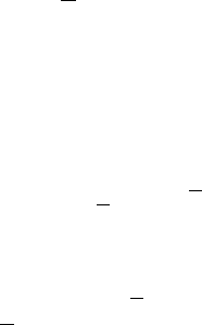
where the nullclines of the kinetics are as shown in Fig. 1.24 (cf. Fig. 1.6). This

system is called an activator–inhibitor system because ∂f /∂ v > 0, thus increased

1.4 Qualitative Methods for Partial Differential Equations 45

Fig. 1.24 Phase diagram for

kinetics of (1.217)

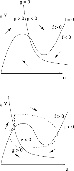
Fig. 1.25 Phase plane for

excitable kinetics

v activates u, while ∂g/∂u < 0, so increased u inhibits v. When the intersection

is on the decreasing part of f = 0, as shown, then ∂f /∂ u > 0, ∂g/∂v < 0, and

−f

> −g

, whence the determinant D of the Jacobian of (u, v)

at the

ﬁxed point is positive. Hence the ﬁxed point is unstable if f

> 0, and a limit

cycle exists in this case if trajectories are bounded. For example, if f =F/ε, ε 1,

this is the case, and the limit cycle takes the relaxational form shown in Fig. 1.6.

The addition of diffusion allows travelling wave trains to exist, as described above.

Solitary Waves in Excitable Media

Suppose now the intersection point of the nullclines f = 0 and g = 0isasshown

in Fig. 1.25. The ﬁxed point of the underlying dynamical system is now stable,

but relatively small perturbations to v can cause large excursions in u,asshown.

When diffusion is included, these large excursions can travel as solitary waves. The

simplest way to understand how this comes about is if we allow u to have fast

reaction kinetics and take v as having zero diffusion coefﬁcient.

46 1 Mathematical Modelling

Fig. 1.26 Phase plane for

solitary wave trajectory

In one dimension, a suitably scaled model is then

εu

=f(u,v)+ε

=g(u,v),

(1.218)

and we look for a travelling wave solution of the form

u =u(ξ), v =v(ξ), ξ = ct −x, (1.219)

where c (assumed positive) is to be found. Then

εcu



=f +ε





=g,

(1.220)

and the idea is to seek a trajectory for which (u, v) →(u

∗

) as ξ →±∞(here

∗

) is the ﬁxed point of the system). The form of this trajectory is shown in

Fig. 1.26. On the slow parts of the wave, f ≈ 0 and cv



≈g. On the fast parts, we put

ξ =εΞ; then v ≈ constant, and we denote v

(=v

∗

) and v

−

as the corresponding

values of v; v

−

is unknown (as is c).

On the fast parts of the wave, we deﬁne u



= w (where now u



= du/dΞ), so

that



=w,



=cw −f

(u),

(1.221)

where f

(u) = f(u,v

). The graphs of f

and f

−

are similar, and are shown in

Fig. 1.27, where we see that construction of the connecting branches PQ and RS

requires that the ﬁxed points P and Q,orR and S,of(1.221) have a connecting

trajectory. In general, this will not be the case, but we can choose c to connect P to

Q (since v

is known), and then we choose v

−

to connect R to S (with this same

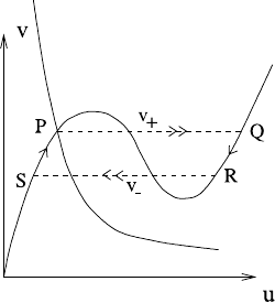
value of c). The form of the resulting travelling wave is shown in Fig. 1.28.

1.4 Qualitative Methods for Partial Differential Equations 47

Fig. 1.27 Phase plane

connection for the fast parts

of the travelling wave

Pattern Formation

We have seen that an activator (v)-inhibitor (u) system

˙u = f(u,v),

˙v =g(u, v),

(1.222)

admits periodic travelling waves when the uniform state is unstable, and solitary

waves when it is stable (and the activator diffuses slowly). Stationary patterns can

occur when a stable steady state of (1.222) is rendered spatially unstable by different

component diffusivities. Suppose that

=f(u,v)+u

=g(u,v) +dv

(1.223)

is an activator–inhibitor system with f

> 0, g

< 0; the restriction to one spatial

dimension is inconsequential. The parameter d here represents the ratio of activator

to inhibitor diffusivities. Note that when d →0, we expect solitary wave propaga-

Fig. 1.28 Spatial form of the

travelling wave

48 1 Mathematical Modelling

tion, at least for the phase diagram of Fig. 1.25, where also f

< 0, g

< 0atthe

ﬁxed point.

With the stationary state denoted as (u

∗

), we assume it is stable in the absence

of diffusion; thus assume

T =f

< 0,

 =f

−f

> 0,

(1.224)

both evaluated at (u

∗

). We put







∗



+we

σt+ikx

; (1.225)

linearisation of (1.223) then yields



M −k

D −σ



w =0, (1.226)

where

M =





,D=



0 d



. (1.227)

The eigenvalues σ are the roots of

−T

σ +

=0, (1.228)

where

=T −(1 +d)k



= −k

(df

) +dk

(1.229)

The steady state is stable if and only if T

< 0 and 

> 0(cf.Fig.1.4). Now T<

0 and >0 by assumption: hence T

< 0, and thus instability occurs if and only if



< 0. Since >0, we see from (1.227) that this can only occur if df

> 0.

Thus either f

> 0org

> 0, and the system cannot be excitable. Since f

< 0,

we see that a necessary condition for instability is that d =1. Because d is the ratio

of two diffusivities, this instability is known as diffusion-driven instability (DDI), or

Turing instability, after the originator of the theory.

To be speciﬁc, let us suppose the situation to be that of Fig. 1.24, i.e., f

> 0,

< 0: then we require d>1 for DDI. The precise criterion for instability is that

min

< 0, and, from (1.229), this is

> 2[d]

1/2

, (1.230)

and this can be reduced to





1/2

+{f

1/2



. (1.231)

1.4 Qualitative Methods for Partial Differential Equations 49

The resulting instability is direct and not oscillatory (in time), though it is oscilla-

tory in space. We can therefore expect stationary ﬁnite amplitude patterns to emerge

as the stable solutions, and this is indeed what often occurs.

The form of these putative steady solutions as d becomes large can be studied by

seeking (spatially) periodic solutions of

+f(u,v)=0,

+ε

g(u,v) =0,

(1.232)

where we deﬁne ε

=1/d 1.

We begin by seeking solutions with period of O(1).Asu varies over distances

of x = O(1), v =¯v is approximately constant, and thus the equation for u can be

integrated to give the ﬁrst integral

+V(u,¯v) =E, (1.233)

where

V(u,v)=



f(u,v)du, (1.234)

and E is constant.

The forms of the curves f(u,v)= 0 (deﬁning v as a function of u), f(u,v) as

a function of u for various ﬁxed v, and V(u,v) as a function of u are shown in

Fig. 1.29. For constant v, solutions for u will be periodic if they lie in the potential

well of V .Given ¯v and E, these periodic solutions are fully determined, and in

particular their period P is a function of ¯v and E, thus P = P(¯v,E). The choice

of ¯v and E must then be made so that v is periodic. We can choose the origin of x

so that u is maximum there; then in fact u is even, and hence so is g[u(x;¯v, E), ¯v].

Integration of (1.232)

then yields

v =¯v −ε



−P/2

(x −ξ)g



u(ξ;¯v, E), ¯v



dξ, (1.235)

where periodicity of v requires that



P/2

−P/2



u(ξ;¯v, E), ¯v



dξ =0. (1.236)

(We also require that



P/2

−P/2

ξg



u(ξ;¯v, E), ¯v



dξ =0, (1.237)

but this is satisﬁed automatically since the integrand is odd.)

Given ¯v,(1.236) appears to determine E, and thus provide a one-parameter fam-

ily of periodic solutions. However, it is unlikely that (1.236) can generally be satis-

ﬁed for a given function g. Consideration of Fig. 1.29 suggests that it is more likely