Fowler A. Mathematical Geoscience
Подождите немного. Документ загружается.

50 1 Mathematical Modelling
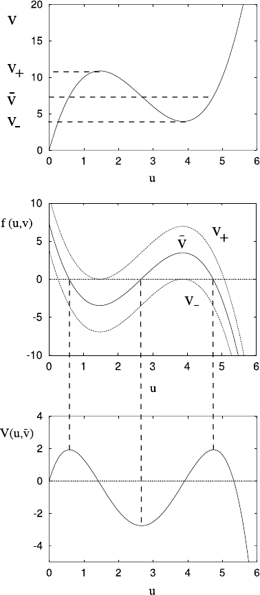
Fig. 1.29 Definition of the
values v
±
defined by the
function f(u,v).Theupper
graph shows the curve
defined implicitly by
f(u,v)= 0 (compare
Fig. 1.24). The middle graph
shows the function f(u,v)as
a function of u for
v =v
+
, ¯v,v
−
,andthelowest
graph is the potential
V(u,v)=
u
0
f(u,v)dufor
the value of v =¯v
corresponding to the middle
of these three curves. The
choice of ¯v in the figure is
that for which the two
maxima of V are equal. The
particular function used in the
illustrations is
f(u,v)= v −[u
3
−8u
2
+17u],
for which the value of ¯v
where the maxima are equal
is ¯v ≈7.407; the values of v
+
and v
−
are v
+
≈10.879 and
v
−
≈3.935
that, given ¯v and E, satisfaction of (1.236) will depend on the precise location of
the curve g =0. For a function g(u,v;α) dependent on a single parameter α, such
as g = α − u
3
v, this suggests that (1.236) may be satisfied (if at all) for a unique
value of α(¯v,E). Since also P =P(¯v,E), this suggests a one-parameter family of
spatially periodic solutions in which P = P(α).
The other possibility for periodic solutions involves the existence of regions in
which u is constant, separated by boundary layers in which u changes rapidly. In
1.4 Qualitative Methods for Partial Differential Equations 51
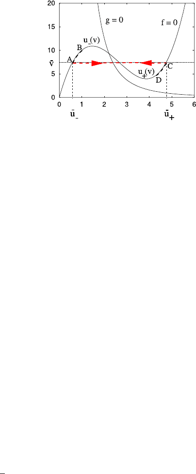
Fig. 1.30 The nullclines
f(u,v)= 0andg(u,v) =0.
The f nullcline defines
locally two functions u
±
(v).
During the oscillation, v
moves from A to B and back
to A,whileg>0, and
similarly from C to D and
back to C while g>0. When
v reaches ¯v, a boundary layer
in u switches the solution
between its two branches
this case, the longer space scale X = εx comes into play, and the resultant form of
Eq. (1.232),
ε
2
u
XX
+f =0,
v
XX
+g =0,
(1.238)
is clearly suggestive of a boundary layer structure.
The boundary layers themselves are still described by (1.233), but now we re-
quire that u tends to constants ¯u
+
and ¯u
−
as x →±∞; this requires ¯v to have the
particular value where the local maxima of V(u,¯v) are the same (and these occur
at ¯u
−
and ¯u
+
). For the value of E equal to this maximum, there are then boundary
layer solutions in which either u goes from ¯u
−
to ¯u
+
as x increases, or from ¯u
+
to ¯u
−
.
The periodic solutions are filled out by solving
v
XX
+g(u,v) =0, (1.239)
in which u is determined by f(u,v)= 0. There are two branches of the resultant
function u(v), which we denote by u
−
(v) and u
+
(v) (and u
±
( ¯v) =¯u
±
), as indicated
in Fig. 1.30; if we define
W(v)=
v
¯v
g[u
−
(v
), v
]dv
for ¯v<v,v
+
,
v
¯v
g[u
+
(v
), v
]dv
for v
−
<v< ¯v,
(1.240)
then W is a V -shaped function defined in [v
−
,v
+
], with a minimum at v =¯v. Solu-
tions for v are determined from
1
2
v
2
X
+W(v)=F, (1.241)
for constant F , and determine a one-parameter family of periodic solutions. Note
that this family occurs for a fixed choice of f and g, and the parameter can be taken
to be the period. This family is then naturally interpreted as the continuation to large
52 1 Mathematical Modelling
d of the bifurcating family dependent on wave number which arises when (1.231)
is satisfied.
1.5 Notes and References
Modelling By mathematical modelling, I mean the formulation of a problem in
mathematical terms. If the process is continuous, usually the model will take the
form of differential equations, and in this book we further confine ourselves to de-
terministic models, as opposed to stochastic models. Stochastic models are of in-
creasing popularity, aiming as they do to represent the noisiness of a system, but
they can also be something of an excuse to sweep things we do not understand un-
der the carpet.
The original classic book which set out the applied mathematician’s stall is that
by Lin and Segel (1974). It contains the ethos of applied mathematics, but retained
a somewhat austere choice of applications. Another classic book which dealt much
more with practical (mostly industrial) applications is that by Tayler (1986). My
own book (Fowler 1997) is in a similar spirit.
These books, certainly the latter two, are aimed at graduate level. There are a
number of books which deal more gently, but still genuinely, with modelling. The
classic of this type is perhaps that by Haberman (1998), a reprinted edition of his
1977 text. More recent books in this direction are those by Fowkes and Mahony
(1994), Howison (2005), and Holmes (2009).
Asymptotics and Perturbation Theory Like modelling, there are many books
on perturbation methods. To my mind, the pre-eminent ones are those by Kevorkian
and Cole (1981), Bender and Orszag (1978) and Hinch (1991). Van Dyke’s (1975)
book is also a classic. Other well known books are those by Nayfeh (1973) and
Holmes (1995).
The flavours of these books are subtly different. Bender and Orszag’s block-
buster, taught at M.I.T. in a one-semester course (the whole book), has as its central
part the asymptotic study of boundary layers. The book has the novelty of giving
many numerical illustrations of how good (or bad) the approximations are, and when
they appear to break down.
Kevorkian and Cole’s book (an expanded edition of Cole’s original 1968 mono-
graph) focusses more on multiple scale methods, and takes these to levels of so-
phistication a good deal beyond more elementary texts, and there are expositions of
some classic problems: the derivation of the Korteweg–de Vries equation describing
long waves in shallow water, and the relaxational van der Pol oscillator, for example.
Van Dyke’s book is slightly more formal in nature, and mostly concerned with
fluid mechanics. It is one of the few places where one can learn the method of
strained coordinates, a method which is particularly useful in dealing with the mo-
tion of margins and fronts. Hinch’s and Nayfeh’s books include a chapter on strained
coordinates also, as well as the other staple contents. Hinch’s is short, to the point,
succinct. Holmes’s book includes a chapter on homogenisation.

1.5 Notes and References 53
Combustion, Non-linear Diffusion and Blow-up Two early accounts of com-
bustion and exothermic reactions are those by Aris (1975) and Buckmaster and
Ludford (1982). The first of these largely deals with reaction in (solid) permeable
catalysts, while combustion theory of the second tends to deal with gaseous com-
bustion, where the theory has all the complication of compressible gas dynamics
together with the species reaction kinetics. A more mathematical book is that by
Bebernes and Eberly (1989). Other books on this subject include those of Williams
(1985), Barnard and Bradley (1985) and Glassman (1987), the latter two more de-
scriptive than Williams’s voluminous work. A similar analytic approach is that by
Liñán and Williams (1993), but this book is more concise than that of Williams.
Combustion really applies to any reaction, but by convention refers specifically to
reactions where there is a large change of temperature. If this is such that the re-
actants become luminous, we have a flame. If the change of temperature is rapid,
we have a thermal explosion. Since in gases, increase of temperature is associated
with increase of pressure, explosions tend to be associated with shock waves, or
detonation waves, and this is the explosive ‘blast’.
The classical treatment of thermal explosions (in solids) is much as described in
Sect. 1.4.8, and involves the positive feedback associated with exothermic reactive
heating, which causes the runaway. Explosive runaway can also be caused by au-
tocatalytic feedback in the reaction scheme, much as in a nuclear explosion; this is
the ‘chain’ reaction. Systems with autocatalysis are also prone to oscillatory bifur-
cations and waves, and are dealt with in the book by Gray and Scott (1990). Ignition
of explosions may be caused by impact or friction (as in striking a match). Both
events cause a localised hotspot to occur, that of impact being due to the sudden
compression of small gas bubbles, see Bowden and Yoffe (1985).
Reactions in a diffusive flame (i.e., one where fuel and oxidant are not pre-mixed)
can be analysed using large activation energy asymptotics; the reactions occur in
a narrow front which spreads as a deflagration wave, whose speed is less than the
sound speed, and is rate-limited by the supply of reactant to the front. The detonation
wave is a reactive shock wave, in which the reaction is triggered not by supply of
reactant, but by gas compression and consequent heating within the shock.
The book by Samarskii et al. (1995) provides a wealth of information about
non-linear diffusion equations, and their associated solution properties of compact
support and blow-up. The asymptotic description given here of the local similarity
structure for the blow-up of solutions of u
t
= u
xx
+ λe
u
is based on that of Dold
(1985).
Burgers’ Equation Burgers’ equation relates to a model introduced by Burgers
(1948) to describe turbulence in fluid flow in a pipe. In its original form, his model
is given by the pair of equations
b
dU
dt
=P −
νU
b
−
1
b
b
0
v
2
dy,
∂v
∂t
+2v
∂v
∂y
=
Uv
b
+ν
∂
2
u
∂y
2
.
(1.242)
54 1 Mathematical Modelling
This is a toy model which aims to mimic the classical procedure of Reynolds aver-
aging, leading to an evolution equation for the mean flow U(t), and another for the
fluctuating velocity field v(y, t). The cross stream variable is y, and the width of the
‘pipe’ is b. Burgers’ equation follows from the assumption that U =0, and arises in
the original paper as an approximation to describe the transition region near shocks;
Burgers gives the travelling wave front solution for this case. A thorough discussion
of Burgers’ equation is given by Whitham (1974).
Fisher’s Equation The geneticist R.A. Fisher wrote down his famous equation
(Fisher 1937) to describe the propagation of an advantageous gene in a population
situated in a one-dimensional continuum—Fisher had in mind a shore line as an
example. The genes (or more properly alleles, i.e., variants of genes), reside in the
members of a population, and the proportion of different alleles of any particular
gene is described by Hardy–Weinberg kinetics. If one allele has a slight evolutionary
advantage, then its proportion p will vary slowly from generation to generation, and
its rate of change is given in certain circumstances by the logistic equation ˙p =
kp(1 −p). The effect of diffusion allows the genes to migrate through the migration
of the carrier population. See Hoppensteadt (1975) for a succinct description. Fisher
did not bother with all this background, but simply wrote his equation down directly.
As well as this paper, he authored or co-authored eight other papers in the same
volume, as well as being the journal editor!
Solitons There are many books on solitons. An accessible introduction is the book
by Drazin and Johnson (1989), and a more advanced treatment is that of Newell
(1985). The subject is rich and fascinating, as is also the curious discovery of the
‘first’ soliton, or ‘great wave of translation’ by John Scott Russell in 1834, as he
followed it on horseback along the Edinburgh to Glasgow canal. The Korteweg–de
Vries equation which appears successfully to describe such waves was introduced
by them much later (Korteweg and de Vries 1895), by which time they are referred to
as solitary waves. Korteweg and de Vries also wrote down the periodic (but unstable)
cnoidal wave solutions.
There are many other equations which are now known to possess soliton solu-
tions, and their folklore has crept into many subjects. Under the guise of ‘magmons’,
for example, they have appeared in the subject of magma transport, which we dis-
cuss in Chap. 9.
Reaction–Diffusion Equations Any book on mathematical biology (and there
are a good number of these) will discuss reaction–diffusion equations. The gold
standard of the type is the book (now in two volumes) by Murray (2002), which also
contains much other subject matter. A more concise book just on reaction–diffusion
equations is that by Grindrod (1991). These books span the undergraduate/graduate
transition. The book by Edelstein-Keshet (2005) is gentler, and aimed at a lower
level.
Kopell and Howard (1973) and Howard and Kopell (1977) studied waves in
reaction–diffusion equations using the ideas of bifurcation theory and multiple

1.6 Exercises 55
scales. Keener (1980, 1986) studied spiral wave formation in excitable media, us-
ing as a template a singularly perturbed pair of equations, essentially of Fitzhugh–
Nagumo type.
Meinhardt (1982) studied pattern formation in reaction–diffusion systems, and
later (Meinhardt 1995) studied the relation between a suite of mathematical models
and actual observed patterns on sea shells. The comparison is striking as well as
pictorially sumptuous.
1.6 Exercises
1.1 Suppose
Pe
∂T
∂t
+u.∇T
=∇
2
T +1inD,
with
T = 0on∂D,
T = ΛΘ(x) in D at t =0,
and Θ = O(1), Λ 1, Pe 1. Discuss appropriate scales for the various
phases of the solution.
1.2 The differential equation
˙x =a −xe
−x
,x>0,a>0,
may have 0, 1 or 2 steady states. Determine how these depend on a, and de-
scribe how solutions behave for a>e
−1
and a<e
−1
, depending on the value
of x(0).
1.3 Each of the equations
z
5
−εz −1 =0,
εz
5
−z −1 = 0,
has five (possibly complex) roots. Find leading order approximations to these
if ε 1. Can you refine the approximations?
1.4 u and v satisfy the ordinary differential equations
˙u = k
1
−k
2
u +k
3
u
2
v,
˙v = k
4
−k
3
u
2
v,
where k
i
> 0. By suitably scaling the equations, show that these can be written
in the dimensionless form
˙u = a −u +u
2
v,
56 1 Mathematical Modelling
˙v = b −u
2
v,
where a and b should be defined. Show that if u, v are initially positive, they
remain so. Draw the nullclines in the positive quadrant, show that there is a
unique steady state and examine its stability. Are periodic solutions likely to
exist?
1.5 The relaxational form of the van der Pol oscillator is
ε ¨x +
x
2
−1
˙x +x =0,ε 1.
A suitable phase plane is spanned by (x, y), where y = ε ˙x +
1
3
x
3
− x.De-
scribe the motion in this phase plane, and find, approximately, the period of
the relaxation oscillation. What happens if ε<0?
1.6 Find a scaling of the combustion equation
c
dT
dt
=−k(T −T
0
) +A exp
−
E
RT
,
so that it can be written in the form
˙
θ =θ
0
−g(θ),
where θ
0
=RT
0
/E and g =θ −αe
−1/θ
. Give the definition of α. Hence show
that the steady state θ is a multiple-valued function of θ
0
if α>
1
4
e
2
.
Find approximations to the smaller and larger positive roots of x
2
e
−x
=ε,
where ε is small and positive. Hence find the approximate range (θ
−
,θ
+
) of
θ
0
for which there are three steady solutions.
Suppose that α>
1
4
e
2
, and θ
0
varies slowly according to
˙
θ
0
=ε(θ
∗
−θ),
where ε 1. Show that there are three possible outcomes, depending on the
value of θ
∗
, and describe them.
1.7 A forced pendulum is modelled by the (dimensional) equation
l
¨
θ +k
˙
θ +g sin θ =α sin λt.
By non-dimensionalising the equation, show how to obtain (1.47), and identify
the parameters ε, β, Ω
0
and ω.
1.8 It is asserted after (1.59) that Ω(A) is a decreasing function of A for 0 <A<
π, or equivalently, that the function
p(A) =
1
√
2
A
0
du
[cosu −cos A]
1/2
is increasing. Show that this is true by writing p in the form
p =
1
0
θ
sinθ
1/2
φ
sin φ
1/2
dw
(1 −w
2
)
1/2

1.6 Exercises 57
for some functions θ(w,A) and φ(w,A), and using the fact that θ/sin θ is an
increasing function of θ in (0,π).
[Hint: cos u −cosA =2sin(
A−u
2
) sin(
A+u
2
).]
1.9 A simple model for the two-phase flow of two fluids along a tube is
α
t
+(αv)
z
=0,
−α
t
+
(1 −α)u
z
=0,
ρ
g
(αv)
t
+
αv
2
z
=−αp
z
,
ρ
l
(1 −α)u
t
+
D
l
(1 −α)u
2
z
=−(1 −α)p
z
,
where p is pressure, u and v are the two fluid velocities, α is the volume
fraction of the fluid with speed v, ρ
g
is its density, and ρ
l
is the density of the
other fluid. Show that there are two characteristic speeds dz/dt =λ, satisfying
(λ −u)
2
=(D
l
−1)
u
2
+2u(λ −u)
−s
2
(λ −v)
2
,
where
s =
ρ
g
(1 −α)
ρ
l
α
1/2
.
Deduce that the characteristic speeds are real if, when D
l
−1 1, s 1,
D
l
>
∼
1 +
s(u −v)
u
2
.
In particular, show that the roots are complex if D
l
=1 and u =v. What does
this suggest concerning the well-posedness of the model?
1.10 The function u(x, t) satisfies
u
t
+uu
x
=α
1 −u
2
for −∞<x<∞, with u =u
0
(x) at t =0, and 0 <u
0
< 1 everywhere. Show
that the characteristic solution can be written parametrically in the form
u =
u
0
(s) +tanh αt
1 +u
0
(s) tanh αt
, exp
α(x −s)
=
sechαt
1 −u tanh αt
.
Sketch the form of the characteristics for an initial function such as u
0
(s) =
a/(1 +s
2
). Show that, in terms of s and t, u
x
is given by
u
x
=
[α sech
2
αt]u
0
(s)
[1 +u
0
(s) tanh αt][α +{u
0
(s) +αu
0
(s)}tanh αt]
,

58 1 Mathematical Modelling
and deduce that a shock will form if u
0
+ α(1 + u
0
) becomes negative for
some s. Show that if u
0
=a/(1 +s
2
) and a is small, this occurs if
α
<
∼
3a
√
3
8
.
1.11 Discuss the formation of shocks and the resulting shock structure for the equa-
tion
u
t
+u
α
u
x
=ε
u
β
u
x
x
,
where α, β > 0, and ε 1. (Assume u>0, and u →0at±∞.)
Show that the equation
u
t
+uu
x
=εuu
xx
admits a shock structure when ε 1, but that the shock speed is not given by
˙x
S
=
1
2
(u
+
+u
−
) (cf. (1.74)). Why should this be so?
1.12 Use phase plane methods to study the existence of travelling wave solutions to
the equation
u
t
=u
p
1 −u
q
+
u
r
u
x
x
,
when (i) p =1, q =2, r =0; (ii) p =1, q =1, r =1.
1.13 Two examples of integrable partial differential equations which admit soliton
solutions are the non-linear Schrödinger (NLS) equation
iu
t
=|u|
2
u +u
xx
,
and the sine-Gordon equation
u
tt
−u
xx
=sin u.
Show that these equations admit solitary wave solutions (which are in fact
solitons).
1.14 Write down the equation satisfied by a similarity solution of the form u =
t
β
f(η), η =x/t
α
, for the equation
u
t
=
u
m
u
x
x
in 0 <x<∞,
where m>0, with u
m
u
x
=−1atx = 0, u → 0asx →∞, u = 0att = 0.
Show that
∞
0
fdη=1, and hence show that in fact f reaches zero at a finite
value η
0
. Is the requirement that m>0 necessary?
1.15 u satisfies the equation
u
t
=
D(u)u
x
x
in 0 <x<∞,
with u =0atx →∞and t =0. For a general function D (not a power of u),
for what kind of boundary condition at x = 0 does a similarity solution exist?
What if, instead, D = D(u
x
)? Write down suitable equations and boundary
conditions for the similarity function in each case.
1.6 Exercises 59
1.16 The depth of a small droplet, h, satisfies the surface-tension controlled equa-
tion
h
t
=−
γ
3μ
∇.
h
3
∇∇
2
h
.
Suppose that a small quantity
hdA=M is released at time zero at the ori-
gin. Find a suitable similarity solution in one and two horizontal spatial di-
mensions.
1.17 A gravity-driven droplet of fluid spreads out on a flat surface. Its viscosity μ is
a function of shear rate, so that a lubrication approximation leads to the model
for its depth h, shear stress τ and velocity u:
ρg∇h =
∂τ
∂z
,
∂u
∂z
=A|τ |
n−1
τ.
(A constant viscosity fluid has n =1.) Show that the horizontal fluid flux is
q =−
A(ρg)
n
n +2
|∇h|
n−1
h
n+2
∇h,
and deduce that
∂h
∂t
=
A(ρg)
n
n +2
∇.
h
n+2
|∇h|
n−1
∇h
.
Non-dimensionalise the model, assuming initial emplacement of a finite vol-
ume M at the origin, and find similarity solutions in one and two dimensions
for the depth. What happens as n →∞or n →0?
1.18 The depth h of a symmetric (two-dimensional) droplet under the influence of
gravity and surface tension is described by the dimensionless equation
∂h
∂t
=
∂
∂x
h
3
∂
∂x
Bh −
∂
2
h
∂x
2
,
subject to the conditions
h =0,h
x
=∓tan θ at x =±x
0
,
x
0
−x
0
hdx =A,
where θ is the contact angle. Show that there is a steady state solution h =
h
0
u(x), in which
1
u
du
[(1 −u)(ρ −u)]
1/2
=
√
B|x|,