Flechtner F.M., Gruber Th., G?ntner A., Mandea M., Rothacher M., Sch?ne T., Wickert J. (Eds.) System Earth via Geodetic-Geophysical Space Techniques
Подождите немного. Документ загружается.


388 W. Freeden et al.
we combine the classical Euclidean wavelets for the time domain with the spherical
wavelets for the space domain and, second, we build up tensor product wavelets with
Legendre wavelets and spherical wavelets for the time and space domain, respec-
tively. The comparison of both wavelet methods is performed in Sect. 3, and we
propose a filtering method for the extraction of an improved hydrological model in
Sect. 4. In the last section some conclusions are drawn.
All computations have been performed based on 62 monthly data sets of spherical
harmonic coefficients up to degree and order 70 from GRACE and WGHM for the
period of August 2002 till September 2007. The data have been provided by our
project partners from the German Centre for Geosciences (GFZ), Department 1:
Geodesy and Remote Sensing.
2 Multiscale Analysis
This section starts with a short introduction to the theory of spherical multiresolu-
tion. For a more detailed representation see Freeden and Michel (2004), Freeden and
Schneider (1998) and Freeden et al. (1998). Let L
2
() be the space of all square-
integrable functions on the unit sphere ,letY
n,m
, n ∈ IN
0
, m = 1, ...,2n + 1,
be an L
2
()-orthonormal system of spherical harmonics. The idea of the spheri-
cal multiscale analysis is to choose kernel functions (so-called scaling functions)
J
(ξ ,η) =
∞
n=0
(
J
)
∧
(n)
2n+1
m=1
Y
n,m
(ξ )Y
n,m
(η) which depend on a scale J ∈ IN
0
in order to build up the scale spaces V
J
=
!
J
∗
J
∗ F
F ∈ L
2
()
"
, where “∗”
denotes the convolution, in such a way that we get a multiresolution (i.e., a nested
sequence of subspaces) of L
2
(): V
0
⊂ ··· ⊂ V
J
⊂ V
J+1
⊂ ··· ⊂ L
2
()
with L
2
() =
∞
%
J=0
V
J
||·||
L
2
()
. The transmission from V
J
to V
J+1
is performed by
use of the detail space W
J
=
!
J
∗
J
∗ F
F ∈ L
2
()
"
via V
J+1
= V
J
+ W
J
,
where the wavelets are given by
J
(ξ ,η) =
∞
n=0
(
J
)
∧
(n)
2n+1
m=1
Y
n,m
(ξ )Y
n,m
(η)
and the symbols of the scaling functions and the wavelets fulfill a scaling equation
of the form
(
J
)
∧
(n)
2
=
(
J+1
)
∧
(n)
2
−
(
J
)
∧
(n)
2
. For the temporal case
(L
2
([ − 1,1])) we transform the spherical multiscale theory using the normalized
Legendre polynomials P
∗
n
, n
∈ IN
0
, instead of the spherical harmonics Y
n,m
.
2.1 Separated Wavelet Analysis with Spherical Wavelets in Space
and Euclidean Wavelets in Time Domain
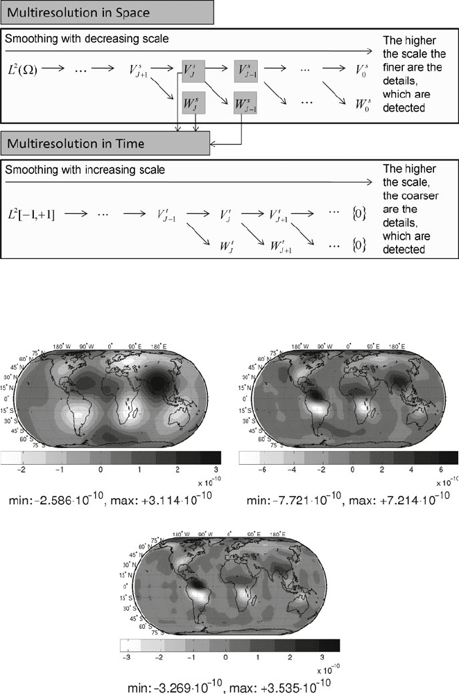
The first idea we follow is to analyze the data in two steps: starting from the original
data a spherical wavelet analysis is performed. The result is a time series of spherical
wavelet coefficients which show more and more (spatial) details with increasing
scale. In the second step we analyze this time series of spherical wavelet coefficients
using Euclidean wavelets and get temporal wavelet coefficients (see Fig. 1). For
the understanding of the classical Euclidean wavelet theory see, e.g., Chui (1992),
Mallat and Hwang (1992) and Mallat and Zhong (1992).
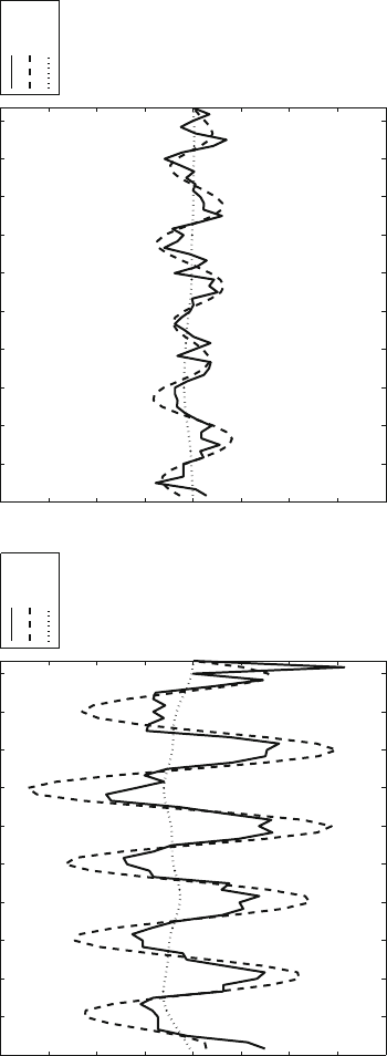
In Figs. 2 and 3 the wavelet coefficients for different scales are presented. The
reader should keep in mind that these coefficients represent the detail information
Time-Space Multiscale Analysis and Its Application to GRACE and Hydrology Data 389
Fig. 1 Separated multiresolution in space and time using spherical and Euclidean wavelets,
respectively
a) spatial scale 2
c) spatial scale 6
b) spatial scale 4
Fig. 2 Space-time wavelet coefficients of GRACE data for April 2005 computed from
spherical c(ubic) p(olynomial)-wavelet coefficients with the quadratic spline wavelet at time
scale 2
390 W. Freeden et al.
Jul02 Jul03 Jul04
a) Manaus (3° S, 60° W)
b) Kaiserslautern (49° N, 7° O)
Jul05 Jul06 Jul07
−2
−1.5
−1
−0.5
0
0.5
1
1.5
2
× 10
−9
scale 0
scale 2
scale 4
Jul02 Jul03 Jul04 Jul05 Jul06 Jul07
−2
−1.5
−1
−0.5
0
0.5
1
1.5
2
× 10
−9
scale 0
scale 2
scale 4
Fig. 3 Time-dependent courses of the space-time wavelet coefficients of the GRACE data in Manaus and Kaiserslautern. For the spatial analysis we used the
cp-wavelet with spatial scale 3 and for the temporal analysis the quadratic spline wavelet for temporal scales 0, 2, 4
Time-Space Multiscale Analysis and Its Application to GRACE and Hydrology Data 391
with whose help we are able to reconstruct the original signal adding detail parts
(following the principle of the multiresolution shown in Fig. 1). In Fig. 2 the
zooming-in effect can be seen clearly: the higher the scale the better the regions
with great changes in the water balance are detected, as, e.g., in the Amazon basin,
Ganges, and Mississippi. In Fig. 3 the time-dependent courses of the space-time
wavelet coefficients in a selected location in the Amazon basin and the correspond-
ing results for Kaiserslautern are shown. In both diagrams we recognize that the
seasonal variations at temporal scale 2 (dimension of the details about 4 months)
can be seen clearly. At time scale 4 (dimension of the details about 16 months) the
course is very smooth, which indicates that it does not make sense to compute higher
scales.
2.2 Tensor Product Wavelets
The principle of the tensor product wavelet analysis which is, e.g., described in
Louis et al. (1998) admits the transmission of the one dimensional multiscale anal-
ysis to higher dimensions. Using the tensor product wavelet theory we are able to
define the multiresolution analysis of the space L
2
([−1,1]×). The theory of spher-
ical wavelets described in Sect. 2 is transformed to the time domain using Legendre
wavelets
J
(s,t) =
∞
n
=0
(
J
)
∧
(n
)P
∗
n
(s)P
∗
n
(t) and the analogously defined tem-
poral scaling functions
J
. As in the spatial case the (temporal) kernel functions
J
and
J
fulfill a scaling equation. Now we are able to build the tensor product
wavelets
˜
i
J
,i=1,2,3, and scaling functions
˜
J
:
˜
i
J
(s,t;ξ ,η) =
∞
n
=0
∞
n=0
2n+1
m=1
(
˜
i
J
)
∧
(n
;n)P
∗
n
(s)P
∗
n
(t)Y
n,m
(ξ )Y
n,m
(η),
˜
J
(s,t;ξ ,η) =
∞
n
=0
∞
n=0
2n+1
m=1
(
˜
J
)
∧
(n
;n)P
∗
n
(s)P
∗
n
(t)Y
n,m
(ξ )Y
n,m
(η),
with the symbols
(
˜
1
J
)
∧
(n
;n) = (
J
)
∧
(n
)(
J
)
∧
(n), (
˜
2
J
)
∧
(n
;n) = (
J
)
∧
(n
)(
J
)
∧
(n),
(
˜
3
J
)
∧
(n
;n) = (
J
)
∧
(n
)(
J
)
∧
(n), (
˜
J
)
∧
(n
;n) = (
J
)
∧
(n
)(
J
)
∧
(n).
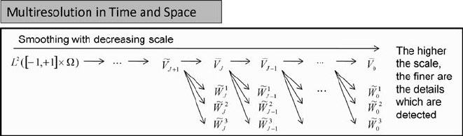
This yields the time-space multiresolution with tensor product wavelets shown
in Fig. 4.
In case of the first hybrid part we smooth in the time domain and detect details
in the space domain, whereas in case of the second hybrid part it is vice versa. The
pure parts in addition show details in both time and space domain. The wavelet
392 W. Freeden et al.
Fig. 4 Multiresolution of L
2
([ −1, + 1] × ) with tensor product wavelets
coefficients of the tensor product multiresolution demonstrate the same structures in
the data sets as shown in Sect. 2.1 for the separated multiresolution using Euclidean
wavelets in the time domain. With increasing scale more and more details can be
recognized in both time and space. A detailed description of the tensor product
wavelet theory and a sound discussion of the results can be found in Nutz and Wolf
(2008).
3 Comparison of the Wavelet Methods Involving
Correlation Coefficients
Considering the computing time we state that the classical Euclidean wavelet trans-
form provides the results time-independent of the scale whereas in case of the
spherical and the tensor product wavelet transform the computing time rises expo-
nentially with increasing scale. Additionally the computing time also depends on
the applied wavelets and for this reason we cannot state in general which method is
faster.
As far as the interpretation of the results is concerned it does not make sense
to directly compare the wavelet coefficients of both methods. This is mainly the
result of the fact that the temporal and spatial details in the first method (Euclidean
wavelets in the time domain) are visualized in different (spatial and temporal) scales,
whereas the second method (tensor product wavelets) has one single scale for both
temporal and spatial analysis which yields the necessity of three different types of
details. Thus we need a tool for the evaluation of the result, and we decided to use
local and global correlation coefficients. Since we average over time the method-
ical differences are diminished and we are able to compare, e.g., the results for
the spatial scales for fixed temporal scale (Euclidean wavelets in the time domain)
with the results for different scales of the pure wavelet coefficients (tensor product
wavelets).
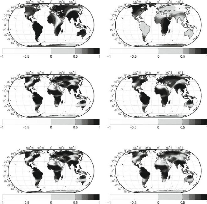
As shown in Fig. 5 we see that the results for both methods are in general quite
similar, as expected, though there are regional differences which have to be inter-
preted in view of an improvement of existing hydrology models. Supplementary,
Time-Space Multiscale Analysis and Its Application to GRACE and Hydrology Data 393
a) spatial scale 2
c) spatial scale 4
c) spatial scale 6
d) scale 4
b) scale 2
f) scale 6
Fig. 5 Local correlation coefficients between GRACE- and WGHM-data computed from wavelet
coefficients with quadratic spline wavelet of scale 2 in the time domain and cp-wavelet of different
scales in the space domain (a, c, e) and from pure tensor product wavelet coefficients with cp-
wavelet of different scales (b, d, f)
Table 1 (a and b) shows the global correlation coefficients for different scales. The
best values are marked in light grey and dark grey.
4 Adapted Filter for the Extraction of a Hydrology Model
from GRACE Data
Our aim now is to interpret the results achieved from the multiscale analysis
with the aid of the correlation coefficients in view of an improvement of exist-
ing hydrology models. To this end we propose a filter based on the correlation

394 W. Freeden et al.
Table 1 Global correlation coefficients for the multiresolution (only on the continents) of GRACE
and WGHM data
(a) Separated wavelet analysis (cp-wavelet in the space domain,
quadratic spline wavelet in the time domain)
(b) Tensor product wavelet analysis with
cp-wavelet in the time and space domain
Temp. scale
Spatial scale 01234Scale
J
∗ F
1
J
∗ F
2
J
∗ F
3
J
∗ F
20.590.79 0.82 0.61 0.29 2 0.04 0.28 0.38 0.38
3
0.68 0.84 0.86 0.66 0.52 3 0.33 0.49 0.58 0.72
4 0.68 0.83 0.85 0.66 0.52 4 0.54 0.51
0.74 0.82
50.65
0.82 0.84 0.64 0.49 5 0.66 0.62 0.74 0.82
6 0.63 0.81 0.83 0.63 0.47 6 0.69
0.66 0.64 0.76
7 0.62 0.80 0.83 0.63 0.47 7 0.68 0.67 0.53 0.66
8 0.62 0.80 0.83 0.62 0.46 8 0.67 0.66 0.46 0.59
coefficients and we assume that we have an improvement if the (global and local)
correlation coefficients of the filtered GRACE and WGHM data are better than
those of the original data. Furthermore we demand that a very large part of the
original signal is reconstructed in the filtered data. Note that the improvement
of the correlation coefficients and the increase of the percentage of the filtered
signal from the original signal cannot be optimized simultaneously. The method
is only applied for the tensor product wavelet analysis but can be transformed
to the separated wavelet analysis with Euclidean wavelets in the time domain,
too.
To find out an optimal filter we start with computing the local correlation coef-
ficients k
(i)
J
on the continents for the corresponding detail parts (of the potential of
GRACE and WGHM) F ∗
(i)
J
∗
(i)
J
and the local correlation coefficients k
J
for
the “reconstructions” F ∗
J
∗
J
. In addition we compute the “global” correla-
tion coefficients gk
(i)
J
,gk
J
. From the correlation coefficients we derive the weights
using a weight function w :[−1,1] → [0,1] which controls the influence of the
corresponding detail part on the resulting reconstructed signal:
F
J
max
=
J
0
∗
J
0
∗ F
(ξ )w
k
J
0
(ξ )
+
J
max
−1
j=J
0
3
i=1
(i)
j
∗
(i)
j
∗ F
(ξ )w
k
(i)
j
(ξ )
.(1)
The weight function is defined by
w(k) =
⎧
⎨
⎩
0, k ≤ G
1
1
G
2
−G
1
k −
G
1
G
2
−G
1
, G
1
< k < G
2
1, k ≥ G
2
,(2)
Time-Space Multiscale Analysis and Its Application to GRACE and Hydrology Data 395
k ∈ [−1,1], with the constants G
1
,G
2
∈ [−1,+1] which help to control the region
of influence: If the correlation coefficient is smaller than G
1
we do not add the
corresponding part in the reconstruction formula (1), whereas in case of a correlation
coefficient greater than G
2
we add the entire part. In case of a correlation coefficient
G
1
< k < G
2
we weight the corresponding part in the reconstruction formula (1) in
such a way that for higher correlation coefficients we use greater weights. In order to
get the percentage of the reconstructed signal F
rec
from the original signal F
orig
we
use the energy which is given by ||F||
2
L
2
([−1,+1]×)
=
∞
n
=0
∞
n=0
∞
m=1
F
∧
n
;n,m
2
for F ∈ L
2
([−1,+1]×), where F
∧
n
;n,m
are the time-space Fourier coefficients.
The percentage p(F
rec
,F
orig
) is then given by
p(F
rec
, F
orig
) =
F
rec
L
2
(−1,+1]×)
&
&
F
orig
&
&
L
2
(−1,+1]×)
.
In analogy we compute the percentage of the detail parts from the total signal.
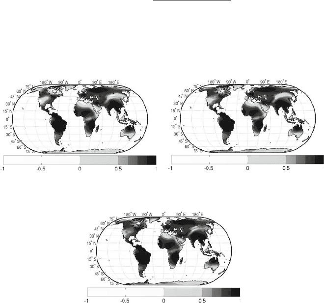
a) Original data (gk = 0.75) b) Reconstruction with G
1
= –0.1 and G
2
= –0.09
(90.04% gk
= 0.81).
b) Reconstruction with G
1
= 0.01 and G
2
= 0.53
(80.03% gk = 0.84).
Fig. 6 Correlation coefficients between the original signals and two reconstructions with details
up to scale 9 from GRACE and WGHM (gk: global correlation coefficient, G
1
and G
2
control the
region of influence of the weight function cf. Eq. (2))

396 W. Freeden et al.
Table 2 Percentage of the reconstruction with details up to scale 9 from GRACE data to the
original GRACE data and correlation coefficients for the corresponding reconstructions between
GRACE and WGHM data for different values of G
1
and G
2
Percentage Corr. coeff. G
1
and G
2
Original (100) 0.75 –
95 0.77 – 0.8 and –0.68
90 0.81 – 0.1 and –0.09
85 0.83 0.1 and 0.22
80 0.84 0.1 and 0.53
In Fig. 6 the correlation coefficients between the original data (Fig. 6a) and for
two reconstructions (Fig. 6b and c) are shown. In addition, Table 2 shows some
more optimal results for different values G
1
and G
2
.
5 Conclusions
A time-space multiscale analysis using two different methods is introduced: First a
separated wavelet concept and, second, a tensor product wavelet concept is realized.
Both methods turn out to be an efficient tool to extract all at once temporally and spa-
tially local phenomena. The results of the multiresolution analysis are finally used
for developing a filter that makes it possible to extract an improved hydrological
model, where we have to be aware of the fact that both a complete reconstruc-
tion of the data and an improvement of the correlation coefficients are mutually
exclusive.
References
1. Chui C (1992) An introduction to wavelets, Academic Press, Boston, MA.
2. Döll P, Kaspar F, Lehner B (2003) A global hydrological model for deriving water availability
indicators: Model tuning and validation. J. Hydrol. 270, 105–134.
3. Fengler M, Freeden W, Kohlhaas A et al. (2007) Wavelet modelling of regional and
temporal variations of the Earth’s gravitational potential observed by GRACE. J. Geod.
81, 5–15.
4. Freeden W (1999) Multiscale modelling of spaceborne geodata, Teubner, Stuttgart, Leipzig.
5. Freeden W, Michel V (2004) Multiscale potential theory (with application to the geoscience),
Birkhäuser, Berlin.
6. Freeden W, Schneider F (1998) An integrated wavelet concept of physical geodesy. J. Geod.
72, 259–281.
7. Freeden W, Schreiner M (2009) Spherical functions of mathematical geosciences, Springer,
Heidelberg.
8. Freeden W, Gervens T, Schreiner M (1998) Constructive approximation on the sphere (with
application to geomathematics), Oxford Science Publication, Clarendon.
9. Louis AK, Maaß P, Rieder A (1998) Wavelets, Teubner, Stuttgart, Leipzig.
10. Mallat S, Hwang WL (1992) Singularity detection and processing with wavelets. IEEE Trans.
Inf. Theory 38(2), 617–643.
Time-Space Multiscale Analysis and Its Application to GRACE and Hydrology Data 397
11. Mallat S, Zhong S (1992) Characterization of signals from multiscale edges. IEEE Trans.
Pattern. Anal. Mach. Intell. 14(7), 710–732.
12. Nutz H, Wolf K (2008) Time-space multiscale analysis by use of tensor product wavelets and
its application to hydrology and GRACE data. Stud. Geophys. Geod. 52, 321–339.
13. Swenson S, Wahr J (2006) Post-processing removal of correlated errors in GRACE data.
Geophys. Res. Lett., doi: 10.1029/2004GL0119920.
14. Swenson S, Wahr J, Milly PC (2003) Estimated accuracies of regional water storage variations
inferred from the gravity recovery and climate experiment (GRACE). Water Resour. Res., doi:
10.1029/2002WR001808.
15. Tapley BD, Bettadpur S, Ries JC et al. (2004a) GRACE measurements of mass variability in
the earth system. Science 305, 503–505.
16. Tapley BD, Bettadpur S, Watkins MM et al. (2004b) The gravity recovery and climate experi-
ment: Mission overview and early results. Geophys. Res. Lett., doi: 10.1029/2004GL019779.