Fishwick P.A. (editor) Handbook of Dynamic System Modeling
Подождите немного. Документ загружается.

24-12 Handbook of Dynamic System Modeling
p
1
p
3
p
2
t
1
t
2
<M1, M2> <J1, J2, J3>
FIGURE 24.8 Colored Petri net model of the manufacturing system.
(corresponding to transitions t
7
−t
12
in Figure 24.7). There are three color sets: SM, SP, and SM ×SP,
where SM ={M1, M2}, SP ={J1, J2, J3}. The color of each node is as follows:
C(p
1
) ={M1, M2}
C(p
2
) ={J1, J2, J3}
C(p
3
) =SM ×SP
C(t
1
) =C(t
2
) =SM ×SP
CPN models can be analyzed through reachability analysis. As for ordinary Petri nets, the basic idea
behind reachability analysis is to construct a reachability graph. Obviously, such a graph may become
very large, even for small CPNs. However, it can be constructed and analyzed totally automatically, and
there exist techniques that make it possible to work with condensed occurrence graphs without losing
analytic power. These techniques build upon equivalence classes. Another option to the CPN model
analysis is simulation. Readers are referred to Jensen (1997) for a detailed description of the concepts,
analysis methods, and practical use of colored Petri nets.
24.8 Timed Petri Nets
The need for including timing variables in the models of various types of dynamic systems is apparent
since these systems are real time in nature. In the real world, almost every event is time related. When a
Petri net contains a time variable, it becomes a timed Petri net (Wang, 1998). The definition of a timed
Petri net consists of three specifications:
•
the topological structure,
•
the labeling of the structure, and
•
firing rules.
The topological structure of a timed Petri net generally takes the form that is used in a conventional
Petri net. The labeling of a timed Petri net consists of assigning numerical values to one or more of the
following things:
•
transitions,
•
places, and
•
arcs connecting the places and transitions.
The firing rules are defined differently depending on the way the Petri net is labeled with time variables. The
firing rules defined for a timed Petri net control the process of moving the tokens around.
The above variations lead to several different types of timed Petri nets. Among them, deterministic
timed Petri nets (DTPNs) (Ramchandani, 1974) and stochastic timed Petri nets (STPNs) (Molloy, 1982;

Petri Nets for Dynamic Event-Driven System Modeling 24-13
Bause and Kritzinger, 2002), in which time variables are associated with transitions, are the two most
widely used extended Petri nets.
24.8.1 Deterministic Timed Petri Nets
The introduction of deterministic time labels into Petri nets was first attempted by Ramchandani (1974).
In his approach, the time labels were placed at each transition, denoting the fact that transitions are often
used to represent actions, and actions take time to complete. The obtained extended Petri nets are called
deterministic timed Petri nets (DTPNs). (Ramamoorthy and Ho, 1980) used such an extended model to
analyze system performance. The method is applicable to a restricted class of systems called decision-free
nets. This class of nets involves neither decisions nor nondeterminism. In structural terms, each place is
connected to the input of no more than one transition, and to the output of no more than one transition.
A DTPN is a six-tuple (P, T, I, O, M
0
, τ), where (P, T, I, O, M
0
)isaPetrinetandτ : T →R
+
a function
that associates transitions with deterministic time delays.
A transition t
i
in a DTPN can fire at time τ if and only if
(1) for any input place p of this transition, there have been the number of tokens equal to the weight of
the directed arc connecting p to t
i
in the input place continuously for the time interval [τ −τ
i
, τ],
where τ
i
is the associated firing time of transition t
i
;
(2) after the transition fires, each of its output places, p, will receive the number of tokens equal to
the weight of the directed arc connecting t
i
to p at time τ.
An important application of DTPN is to calculate the cycle time of a Petri net model. For a decision-
free Petri net where every place has exactly one input arc and one output arc, the minimum cycle time
(maximum performance) C is given by
C = max
T
k
N
k
: k = 1, 2, , q
where T
k
=
t
i
∈L
k
τ
i
is the sum of the execution times of the transitions in circuit k; N
k
=
p
i
∈L
k
M(p
i
)
the total number of tokens in the places in circuit k; and q the number of circuits in the net.
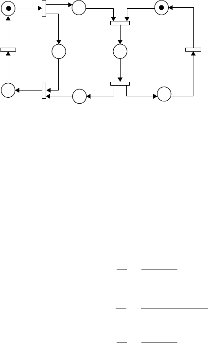
Example 6
A communication protocol.
Consider the communication protocol between two processes, one indicated as the sender and the other
as the receiver. The sender sends messages to a buffer, while the receiver picks up messages from the
buffer. When it gets a message, the receiver sends an acknowledgment (ACK) back to the sender. After
receiving the ACK from the receiver, the sender begins processing and sending a new message. Suppose
that the sender takes 1 time unit to send a message to the buffer, 1 time unit to receive the ACK, and 3
time units to process a new message. Then, the receiver takes 1 time unit to get the messages from the
buffer, 1 time unit to send back an ACK to the buffer, and 4 time units to process a received message.
The DTPN model of this protocol is shown in Figure 24.9. The legends of places and transitions and
timing properties are as follows:
p
1
: The sender ready.
p
2
: Message in the buffer.
p
3
: The sender waiting for ACK.
p
4
: Message received.
p
5
: The receiver ready.
p
6
: ACK sent.
p
7
: ACK in the buffer.
p
8
: ACK received.
24-14 Handbook of Dynamic System Modeling
p
1
p
2
p
5
p
3
p
4
p
6
p
8
t
1
t
2
t
3
t
4
t
6
t
5
p
7
FIGURE 24.9 Petri net model of a simple communication protocol.
t
1
: The sender sends a message to the buffer. Time delay: 1 time unit.
t
2
: The receiver gets the messages from the buffer. Time delay: 1 time unit.
t
3
: The receiver sends back an ACK to the buffer. Time delay: 1 time unit.
t
4
: The receiver processes the message. Time delay: 4 time units.
t
5
: The sender receives the ACK. Time delay: 1 time unit.
t
6
: The sender processes a new message. Time delay: 3 time units.
There are three circuits in the model. The cycle time of each circuit is calculated as follows:
circuit p
1
t
1
p
3
t
5
p
8
t
6
p
1
: C
1
=
T
1
N
1
=
1 +1 +3
1
= 5
circuit p
1
t
1
p
2
t
2
p
4
t
3
p
7
t
5
p
8
t
6
p
1
: C
2
=
T
2
N
2
=
1 +1 +1 + 1 + 3
1
= 7
circuit p
5
t
2
p
4
t
3
p
6
t
4
p
5
: C
3
=
T
3
N
3
=
1 +1 +4
1
= 6
After enumerating all circuits in the net, we know the minimum cycle time of the protocol between the
two processes is 7 time units.
24.8.2 Stochastic Timed Petri Nets
STPNs are Petri nets in which stochastic firing times are associated with transitions. An STPN is essen-
tially a high-level model that generates a stochastic process. STPN-based performance evaluation basically
comprises modeling the given system by an STPN and automatically generating the stochastic process
that governs the system behavior. This stochastic process is then analyzed using known techniques (Haas,
2002). STPNs are a graphical model and offer great convenience to a modeler in arriving at a credible,
high-level model of a system.
The simplest choice for the individual distributions of transition firing times is negative exponential
distribution. Because of the memoryless property of this distribution, the stochastic process associated
with the STPN is a continuous-time homogeneous Markov chain (Ethier, 2005) with state space in one-
to-one correspondences with marking in R(M
0
), the set of all reachable markings. The transition rate
matrix of the Markov chain can be easily constructed from the reachability graph given the firing rates
of the transitions of the STPN. Exponential timed stochastic Petri nets, often called stochastic Petri nets
(SPNs), were independently proposed by Natkin (1980) and Molloy (1981), and their capabilities in the
performance analysis of real systems have been investigated by many authors.
Petri Nets for Dynamic Event-Driven System Modeling 24-15
An SPN is a six-tuple (P, T, I, O, M
0
, ), where (P, T, I, O, M
0
)isaPetrinetand : T →R asetof
firing rates whose entry λ
k
is the rate of the exponential individual firing time distribution associated
with transition t
k
. Natkin and Molloy have shown that the marking process of an SPN is a continuous-
time Markov chain. The state space of the Markov chain is the reachable set R(M
0
). Suppose there are
s markings in R(M
0
), and the underlying Markov chain is ergodic, then the steady-state probability
distribution =(π
0
, π
1
,…,π
s
) can be obtained by resolving the following linear system:
Q = 0
j
π
j
= 1, π
j
≥ 0, j = 0, 1, 2, ...
whereQ is a transitionrate matrixwhose elements outside the main diagonal are the rates of the exponential
distributions associated with the transitions from state, while the elements on the main diagonal make
the sum of the elements of each row equal to zero. Denote by E(M
i
) the set of all enabled transition at
marking M
i
, and T
ij
the set of enabled transitions at marking M
i
whose firings lead the SPN to another
marking M
j
. Then Q is determined as follows:
q
ij
=
t
k
∈T
ij
λ
k
q
i
= q
ii
=−
t
k
∈E(M
i
)
λ
k
The probability of marking M
i
changing to M
j
is the same as the probability that one of the transitions
in the set T
ij
fires before any of the transitions in the set T\T
ij
. Since the firing times in an SPN are mutually
independent exponential random variables, it follows that the required probability has the specific value
given by
α
ij
= q
ij
/q
i
In the expression for α
ij
deduced above, note that the numerator is the sum of the rates of those enabled
transitions in M
i
, the firing of any of which changes the marking from M
i
to M
j
; whereas the denominator
is the sum of the rates of all the enabled transitions in M
i
. Also note that α
ij
=1 if and only if T
ij
=E(M
i
).
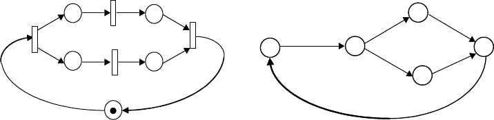
Example 7
A stochastic Petri net.
Figure 24.10 shows a simple SPN model with its reachable markings and its reachable graph. The linear
system of steady-state probabilities is
π
0
+π
1
+π
2
+π
3
+π
4
= 1
Let =(1 1 1 1), then solution to this system is
π
0
= π
4
= 2/7, π
1
= π
2
= π
3
= 1/7
p
1
p
2
p
3
p
4
p
5
t
1
t
2
t
3
t
4
(a)
M
0
M
1
M
2
M
3
M
4
t
1
t
2
t
3
t
3
t
2
t
4
(b)
FIGURE 24.10 (a) SPN model. (b) Reachability graph.

24-16 Handbook of Dynamic System Modeling
The analysis of an SPN model is usually aimed at the computation of more aggregate performance
indices than the probabilities of individual markings. Several kinds of aggregate results are easily
obtained from the steady-state distribution over reachable markings. In this section, we quote some
of the most commonly and easily computed aggregate steady-state performance parameters (Ajmone
Marsan, 1990).
•
The probability of an event defined through place markings (e.g., no token in a subset of places,
or at least one token in a place while another one is empty), can be computed by adding the
probabilities of all markings in which the condition corresponding to the event definition holds.
Thus, for example, the steady-state probability of the event A defined through a condition that holds
for the markings M
i
∈H is obtained as
P{A}=
M
i
∈H
π
i
•
The average number of tokens in a place can be obtained by computing the individual probabilities
as those of the event “place p
i
contains k tokens.”
•
The frequency of firing a transition, i.e., the average number of times the transition fires in unit
time, can be computed as the weighted sum of the transition firing rate:
f
i
=
i:t
j
∈E(M
i
)
λ
j
(M
i
)π
i
where f
j
is the frequency of firing t
j
and λ
j
(M
i
) the firing rate of t
j
at M
i
.
•
The average delay of a token in traversing a subnet in steady-state conditions can be computed using
Little’s formula
E(T) =
E(N)
E(γ)
where E(T) is the average delay, E(N) the average number of tokens in the process of traversing
the subnet, and E(γ) the average input (or output) rate of tokens into (or out of) the subnet. This
procedure can be applied whenever the interesting tokens can be identified inside the subnet (which
can also comprise other tokens defining its internal condition, but these must be distinguishable
from those whose delay is studied) so that their average number can be computed, and a relation
can be established between input and output tokens (e.g., one output token for each input token).
24.9 Concluding Remark
Petri nets have been proven to be a powerful modeling tool for various types of dynamic event-driven
systems. Since Petri nets were introduced in 1962, numerous research papers have been published. The
research has been conducted in many branches, with each branch exploring a promising application aspect
of this formalism. Given the rich research results from the Petri net society, it is hard to cover all of them in
such a short book chapter. Therefore, this chapter only aims at briefly introducing the most basic concepts,
theory and applications of ordinary Petri nets, and a few of the most popular extended Petri nets.
References
Ajmone Marsan, M. 1990. Stochastic Petri nets: An elementary introduction. Advances in Petri Nets,
Lecture Notes in Computer Science 424.
Ajmone Marsan, M., M.G. Balbo, and G. Conte. 1986. Performance Models of Multiprocessor Systems.
Cambridge, MA: MIT Press.
Petri Nets for Dynamic Event-Driven System Modeling 24-17
Andreadakis, S.K. and A.H. Levis. 1988. Synthesis of distributed command and control for the outer air
battle. Proceedings of the 1988 Symposium on C
2
Research, SAIC, McLean, VA.
Bause, F. and P. Kritzinger. 2002. Stochastic Petri Nets—An Introduction to the Theory. Germany: Vieweg
Verlag.
Desrochers, A. and R. Ai-Jaar. 1995. Applications of Petri Nets in Manufacturing Systems: Modeling, Control
and Performance Analysis. New York: IEEE Press.
Ethier, S. N. 2005. Markov Processes. New York: Wiley.
Genrich, J.H. and K. Lautenbach. 1981. System modeling with high-level Petri nets. Theoretical Computer
Science 13: 109–136.
Haas, P. 2002. Stochastic Petri Nets: Modelling, Stability, Simulation. New York: Springer.
Jensen, K. 1981. Colored Petri nets and the invariant-method. Theoretical Computer Science 14: 317–336.
Jensen, K. 1997. Coloured Petri Nets. Basic Concepts, Analysis Methods and Practical Use (3 volumes).
London: Springer.
Lin, C., L. Tian, and Y. Wei. 2002. Performance equivalent analysis of workflow systems. Journal of Software
13(8): 1472–1480.
Mandrioli, D., A. Morzenti, M. Pezze, P. San Pietro, and S. Silva. 1996. A Petri net and logic approach to
the specification and verification of real time systems. In: Formal Methods for Real Time Computing
(C. Heitmeyer and D. Mandrioli, eds.). New York: Wiley.
Memmi, G. and G. Roucairol. 1980. Linear algebra in net theory. Lecture Notes in Computer Science, 84:
213–223.
Merlin, P. and D. Farber. 1976. Recoverability of communication protocols—Implication of a theoretical
study. IEEE Transactions on Communications 1036–1043.
Molloy, M. 1981. On the Integration of Delay and Throughput Measures in Distributed Processing Models.
Ph.D. Thesis, UCLA, Los Angeles, CA.
Molloy, M. 1982. Performance analysis using stochastic Petri nets. IEEE Transactions on Computers 31(9):
913–917.
Murata, T. 1989. Petri nets: Properties, analysis and applications. Proceedings of the IEEE 77(4): 541–580.
Natkin, S. 1980. Les Reseaux de Petri Stochastiques et Leur Application a I’evaluation des Systems
Informatiques. These de Docteur Ingegneur, Cnam, Paris, France.
Peterson, J.L. 1981. Petri Net Theory and the Modeling of Systems. New Jersey: Prentice-Hall.
Petri, C.A. 1962. Kommunikation mit Automaten. English Translation, 1966: Communication with
Automata, Technical Report RADC-TR-65-377, Rome Air Dev. Center, New York.
Ramchandani, C. 1974. Analysis of Asynchronous Concurrent Systems by Petri Nets. Project MAC, TR-120,
MIT, Cambridge, MA.
Ramamoorthy, C. and G. Ho. 1980. Performance evaluation of asynchronous concurrent systems using
Petri nets. IEEE Transaction on Software Engineering 6(5): 440–449.
Tsai, J., S. Yang, and Y. Chang. 1995. Timing constraint Petri nets and their application to schedulability
analysis of real-time system specifications. IEEE Transactions on Software Engineering 21(1): 32–49.
van der Aalst, W. and K. van Hee. 2000. Workflow Management: Models, Methods, and Systems. Cambridge,
MA: MIT Press.
van Landeghem, R. and C.-V. Bobeanu. 2002. Formal modeling of supply chain: An incremental approach
using Petri nets. 14th European Simulations Symposium and Exhibition, Dresden, Germany.
Wang, J. 1998. Timed Petri Nets, Theory and Application. Boston, MA: Kluwer.
Wang, J.,Y. Deng and M. Zhou, 2000. Compositional time Petrinets and reduction rules. IEEE Transactions
on Systems, Man and Cybernetics, Part B, 30(4): 562–572.
Venkatesh, K., M.C. Zhou, and R. Caudill. 1994. Comparing ladder logic diagrams and Petri nets for
sequence controller design through a discrete manufacturing system. IEEE Transaction on Industrial
Electronics 41(6): 611–619.
Zhou, M.C. and F. DiCesare. 1989. Adaptive design of Petri net controllers for error recovery in automated
manufacturing systems. IEEE Transactions on Systems, Man, and Cybernetics
19(5): 963–973.

25
Queueing System Models
Christos G. Cassandras
Boston University
25.1 Introduction ................................................................ 25-1
25.2 Specification of Queueing System Models ................ 25-2
25.3 Performance of a Queueing System ........................... 25-4
25.4 Queueing System Dynamics ....................................... 25-6
25.5 Little’s Law ................................................................... 25-7
25.6 Simple Markovian Queueing Models ........................ 25-8
The M/M/1 Queueing System
25.7 Markovian Queueing Networks ................................. 25-11
The Departure Process of the M/M/1 Queueing
System
•
Open Queueing Networks
•
Closed
Queueing Networks
•
ProductFormNetworks
25.8 Non-Markovian Queueing Systems ........................... 25-17
25.1 Introduction
In a separate chapter, models for discrete-event systems (DES) were introduced and discussed. To briefly
recap, the behavior of such systems is governed by discrete events occurring asynchronously over time and
solely responsible for generating state transitions. In between event occurrences, the state of such systems
is unaffected. Examples include computer and communication networks, automated manufacturing sys-
tems, air traffic control systems, command-control systems, advanced monitoring and control systems in
automobiles or large buildings, intelligent transportation systems, distributed software systems, and so
forth. DES are also referred to as event-driven systems to distinguish them from time-driven systems. In the
latter, the state of the system generally changes as time changes: with every“tick”of an underlying clock the
state is expected to change and differential (or difference) equations are the standard modeling framework
one uses in such cases. In contrast, in an event-driven system state transitions are the result of combining
asynchronous concurrent event processes. Modeling frameworks for DES include state automata and Petri
nets, discussed elsewhere in the book.
An important class of DES is that of queueing systems. The term “queueing” is associated with the fact
that the resources we need to use in most systems we design and build (as well as in our daily life) are
not always accessible: to use them, we have to wait. For example, to use the resource “bank teller” in a
bank, people form a line and wait for their turn. Sometimes, the waiting is not done by people, but by
discrete objects or more abstract“entities.” For example, to use the resource “CPU” in a computer, various
“tasks” wait somewhere until they are given access to it through potentially complex mechanisms. There
are three basic elements that comprise a queueing system: (i) The entities that do the waiting in their quest
for resources; these are traditionally referred to as customers. (ii) The resources for which the waiting is
done; since resources typically provide some form of service to the customers, we shall generically call
them servers; and (iii) The space where the waiting is done, which we shall call a queue.
The study of queueing systems is motivated by the simple fact that resources are not unlimited; if they
were, no waiting would ever occur. This fact gives rise to obvious problems of resource allocation and
related tradeoffs so that (i) customer needs are adequately satisfied, (ii) resource access is provided in fair
25-1
25-2 Handbook of Dynamic System Modeling
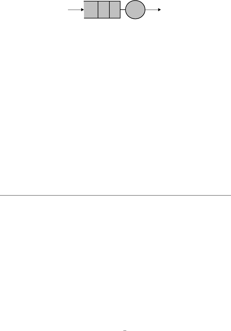
Queue
Server
Customer
arrivals
Customer
arrivals
Customer
departures
FIGURE 25.1 A simple queueing system.
and efficient ways among different customers, and (iii) the cost of designing and operating the system is
maintained at acceptable levels.
Graphically, we will represent a simple queueing system as shown in Figure 25.1. A circle represents
a server, and an open box represents a queue preceding this server. The slots in the queue are meant to
indicate waiting customers. Customers are thought of as arriving at the queue, and departing from the
server. The process of serving customers takes a positive amount of time (otherwise there would be no
waiting). Thus, a server may be thought of as a “delay block,” which holds a customer for some amount of
service time.
Queueing theory is a subject to which many books have been devoted. It ranges from the study of
simple single-server systems modeled as birth–death Markov chains to the analysis of arbitrarily complex
networks of queues. In this chapter, we limit ourselves to the essential ideas and techniques that are used
to analyze simple queueing systems. Queueing theory has as its main goal the determination of a system’s
performance under certain operating conditions, rather than the determination of the operating policies to
be used to achieve the best possible performance. Thus, its mission has been largely to develop“descriptive”
tools for studying queueing systems, rather than “prescriptive” tools for controlling their behavior in an
ever-changing dynamic and uncertain environment. Still, we must stress that queueing theory has made
some of the most important contributions to the analysis of stochastic DES where resource contention
issues are predominant.
25.2 Specification of Queueing System Models
There are three basic aspects of a queueing model that require specification: (i) stochastic models for the
arrival and service processes; (ii) structural parameters of the system, e.g., the storage capacity of a queue
and the number of servers; and (iii) Operating policies, e.g., conditions under which arriving customers
are accepted and preferential treatment (prioritization) of some types of customers by the server.
Stochastic Models for Arrival and Service Processes. Viewed as a DES, the simple model of Figure 25.1
has an event set E ={a, d},wherea denotes a customer arrival and d a departure following a service
completion. We associate with arrival events a a stochastic sequence {Y
1
, Y
2
, ...},whereY
k
is the kth
interarrival time, i.e., the time elapsed between the (k −1)th and kth arrival, k =1, 2, .... For simplicity,
we always set Y
0
=0, so that Y
1
is the random variable describing the time of the first arrival. In most simple
queueing models, it is assumed that the stochastic sequence {Y
k
} is iid (i.e., Y
1
, Y
2
, ... are independent
and identically distributed). Therefore, a single probability distribution
A(t) = P[Y ≤ t] (25.1)
completely describes the interarrival time sequence. In Eq. (25.1), the random variable Y is often thought
of as a “generic” interarrival time that does not need to be indexed by k. The mean of the distribution
function A(t), E[Y], is particularly important and it is customary to use the notation
E[Y] ≡
1
λ
(25.2)
to represent it. Thus, λ is the arrival rate of customers.

Queueing System Models 25-3
Similarly, we associate to the event d a stochastic sequence {Z
1
, Z
2
, ...},whereZ
k
is the kth service time,
i.e., the time required for the kth customer to be served, k =1, 2, .... If we assume that the stochastic
sequence {Z
k
}is also iid, then we define
B(t) = P[Z ≤ t] (25.3)
where Z is a generic service time. Similar to Eq. (25.2), we use the following notation for the mean
of B(t):
E[Z] ≡
1
µ
(25.4)
so that µ is the service rate of the server in our model.
Structural Parameters. The most common structural parameters of interest in a queueing system are (i)
The storage capacity of the queue, usually denoted by K =1, 2, ....By convention, we normally agree to
include in this storage capacity the space provided for customers in service. (ii) The number of servers,
usually denoted by m =1, 2, ....In the simple system of Figure 25.1, we have K =∞and m =1.
Operating Policies. Even for the simple system of Figure 25.1, there are various schemes one can adopt in
handling the queueing process. Here are just some of the natural questions that arise about the operation
of the system: (i) Is the service time distribution the same for all arriving customers? (ii) Are customers
differentiated on the basis of belonging to different“classes,” some of which may have a higher priority than
others in requesting service? (iii) Are all customers admitted to the system? (iv) Are customers allowed to
leave the queue before they get served, and, if so, under what conditions? (v) How does the server decide
which customer to serve next (if there are more than one in the queue); for example, the first one in queue,
anyone at random, and so forth? (vi) Is the server allowed to preempt a customer in service to serve a
higher-priority customer that just arrived?
Clearly, operatingpoliciescan cover a widerange of possibilities. In categorizing them, the most common
issues we consider are the following: (i) Number of customer classes. In the case of a single-class system, all
customers have the same service requirements and the server treats them all equally. This means that the
service time distribution is the same for all customers. In the case of a multiple-class system, customers
are distinguished according to their service requirements and/or the way in which the server treats them.
(ii) Scheduling policies. In a multiple-class system, the server must decide upon a service completion which
class to process next. For example, the server may always give priority to a particular class, or it may
preempt a customer in process because a higher priority customer just arrived. (iii) Queueing disciplines.
A queueing discipline describes the order in which the server selects customers to be processed, even if
there is only a single class. For example, first-come-first-served (FCFS), last-come-last-served (LCFS), and
random order. (iv) Admission policies. Even if a queue has infinite storage capacity, it may be desirable
to deny admission to some arriving customers. In the case of two arriving classes, for instance, higher
priority customers may always be admitted, but lower priority customers may only be admitted if the
queue is empty or if some amount of time has elapsed since such a customer was admitted. (v) Batching.
It is possible that arrivals occur in “batches,” i.e., customers may arrive one at a time or in groups of size
n > 1. Similarly, it is possible that service occurs in batches of size n > 1 customers processed at a time.
In the simple case of Figure 25.1, we assume a single-class system with all arriving customers admitted
and served one at a time and the queueing discipline is FCFS.
Notation. It is customary in queueing theory to employ a particular type of notation to succinctly
describe a system. This notation (attributed to Kendall) is A/B/m/K,whereA is the interarrival time
distribution, B the service time distribution, m the number of servers present, m =1, 2, ..., and K the
storage capacity of the queue, K =1, 2, .... Thus, the infinite queueing capacity single-server system of
Figure 25.1 is described by A/
B/1/∞. To simplify the notation, if the K position is omitted it is understood
that K =∞. Therefore, in our case, we have A/B/1. Furthermore, there is some common notation used
to represent the distributions A and B. In particular, G stands for a General distribution when nothing
else is known about the arrival/service process, GI for a General distribution in a renewal arrival/service
process (i.e., all interarrival/service times in that process are iid), D for the Deterministic case, (i.e., the