Fishwick P.A. (editor) Handbook of Dynamic System Modeling

Подождите немного. Документ загружается.

25-4 Handbook of Dynamic System Modeling

interarrival/service times are ﬁxed), and M for the Markovian case, i.e., the interarrival/service times are

exponentially distributed; using our notation in Eqs. (25.1)–(25.4), this means that A(t) =1 −e

−λt

and

B(t) =1 −e

−µt

These are the most often encountered cases. Here are some examples to illustrate the A/B/m/K notation:

the M/M/1 queueing system has a single server and inﬁnite storage capacity with both interarrival and

service times exponentially distributed; the M/M/1/K system is the same but with storage capacity

givenbysomeK < ∞ (including space at the server); the M/G/2 system has two servers and inﬁnite

storage capacity, with exponentially distributed interarrival times, while the service times have an arbitrary

(general) distribution.

Note that the A/B/m/K notation does not specify the operating policies to be used. It also does

not describe the case where two or more customer classes are present, each with different interarrival and

service time distributions. Finally, note that when A(t) =1 −e

−λt

the underlying arrival process is Poisson.

Thus, the statement “the arrival process is Poisson” is the same as “interarrival times are independent and

exponentially distributed.” In the case of departure events generated by a Poisson process, we normally

use the statement“service times are exponentially distributed,” because these events are only feasible when

the server is busy.

The A/B/m/K notation can be extended to include one more characteristic of a queueing system:

whether it is open to an inﬁnite population of customers who can request service at any time or whether

the system is limited to a ﬁnite population of customers, usually denoted by N. In the latter case, a

customer completing service at some server is always routed to another queue and never leaves the system.

We refer to the former as an open queueing system and the latter as a closed one. In such cases, the notation

A/B/m/K/N is used, where N represents the customer population residing in the system. As in the case

of inﬁnite storage, omitting N implies an open system (i.e., N =∞). Note that if K =∞, but N < ∞,we

normally write A/B/m//N. Closed queueing systems should not be thought of as strictly consisting of a

particular set of ﬁxed customers. Instead, the population N may indicate a number of resources limiting

access to more customers. A typical example arises in modeling a computer system with N access points.

Here, the total number of users is limited to N, but users certainly come and go replacing each other at

various access points. Similarly, in a manufacturing system production parts are often carried in pallets

whose number is limited to N. When a ﬁnished part leaves the system, it relinquishes its pallet to a new

part, so that the effective number of customers in the system is limited to N.

25.3 Performance of a Queueing System

In addition to the random variables already introduced, i.e., the interarrival time Y

and the service time Z

let us deﬁne A

to be the arrival time of the kth customer, D

its departure time, W

its waiting time, and

its system time (from arrival instant until departure), also referred to as response time, sojourn time,or

delay. Note that

= D

−A

= W

(25.5)

and

= A

(25.6)

In addition, we deﬁne the random variables X(t) to denote the queue length at time t, X(t) ∈{0, 1, 2, ...}

and U(t) to denote the workload (or unﬁnished work)attimet, i.e., the amount of time required to empty

the system at t.

The stochastic behavior of the waiting time sequence {W

} provides important information regarding

the system’s performance. The probability distribution function of {W

}, P[W

≤t], generally depends

on k. We often ﬁnd, however, that as k →∞there exists a stationary distribution, P[W ≤t], independent

of k, such that

lim

k→∞

P[W

≤ t] = P[W ≤ t] (25.7)

Queueing System Models 25-5

If this limit indeed exists, the random variable W describes the waiting time of a typical customer at steady

state. Intuitively, when the system runs for a sufﬁciently long period of time (equivalently, the system

has processed a sufﬁciently large number of customers), every new customer experiences a “stochastically

identical” waiting process described by P[W ≤t]. The mean of this distribution, E[W], represents the

average waiting time at steady state. Similarly, if a stationary distribution exists for the system time

sequence {S

}, then its mean, E[S], is the average system time at steady state.

The same idea applies to the stochastic processes {X(t)} and {U(t)}. If stationary distributions exist for

these processes as t →∞, then the random variables X and U are used to describe the queue length and

workload of the system at steady state. We will use the notation π

, n = 0, 1, ..., to denote the stationary

queue length probability, that is,

= P[X = n], n = 0, 1, ... (25.8)

Accordingly, E[X]istheaverage queue length at steady state, and E[U] the average workload at steady state.

In general, we want to design a queueing system so that a typical customer at steady state waits as little

as possible (ideally, zero). In contrast, we also wish to serve as many customers as possible by keeping the

server as busy as possible, that is, we try to maximize the server’s utilization. To do so, we must constantly

keep the queue nonempty; in fact, we should make sure there are always a few customers to serve in case

several service times in a row turn out to be short. However, this is directly contrary to our objective

of achieving zero waiting time for customers. This informal argument serves to illustrate a fundamental

performance tradeoff in all queueing systems. To keep a server highly utilized we must be prepared to

tolerate long waiting times; conversely, to maintain low waiting times we have to tolerate some server

idling. With this observation in mind, the main measures of performance (at steady state) that we are

interested in are (i) the average waiting time of customers, E[W], (ii) the average queue length, E[X],

(iii) the utilization of the system, i.e., the fraction of time that the server is busy, and (iv) the throughput

of the system, i.e., the rate at which customers leave after service. Our objective is to keep the ﬁrst two as

small as possible, while keeping the last two as large as possible.

To gain some more insight on the utilization of a queueing system, we deﬁne the trafﬁc intensity ρ as

ρ ≡

[arrival rate]

[service rate]

Then, by the deﬁnitions of λ and µ in Eq. (25.2) and Eq. (25.4), we have

ρ =

(25.9)

In the case of m servers, the average service rate becomes mµ, and, therefore,

ρ =

mµ

(25.10)

In a single-server system at steady state, the probability π

, deﬁned in Eq. (25.8), represents the fraction of

time the system is empty, and hence the server is idle. It follows that for a server at steady state:

[utilization] ≡ [fraction of time server is busy] = 1 −π

Sinceaserveroperatesatrateµ and the fraction of time that it is actually in operation is (1 −π

), the

throughput of a single-server system at steady state is

[throughput] ≡ [departure rate of customers after service] = µ(1 −π

)

At steady state, the customer ﬂows into and out of the system must be balanced, that is,

λ = µ(1 −π

)

It then follows from Eq. (25.9) that

ρ = 1 −π

(25.11)

25-6 Handbook of Dynamic System Modeling

Thus, the trafﬁc intensity, which is deﬁned by the parameters of the service and interarrival time distri-

butions, also represents the utilization of the system. This relationship holds for any single-server system

with inﬁnite storage capacity. Note that if π

=0, the system is permanently busy, which generally leads to

an instability in the sense that the queue length grows to inﬁnity. Thus, the values of ρ must be such that

0 ≤ρ<1.

A typical design problem for queueing systems is the selection of parameters such as the service

rate and number of servers to achieve some desirable performance in terms of the measures above.

In controlling queueing systems, our task is to select operating policies that help us achieve such

performance.

25.4 Queueing System Dynamics

Consider once again the queueing system of Figure 25.1, operating on an FCFS basis. Using the notation

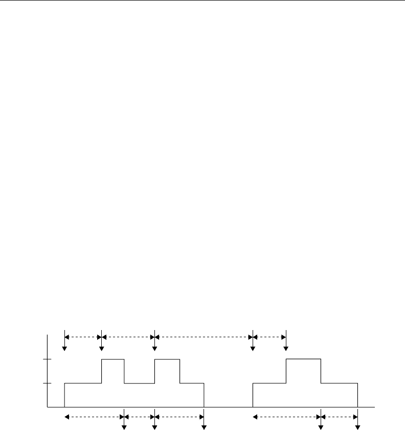
we have established, a typical sample path of this system is shown in Figure 25.2. In this example, the ﬁrst

arriving customer at time A

ﬁnds an empty queue. During the interval starting at A

and ending with

the server remains busy. Such an interval is termed a busy period of the queueing system. During the

interval starting with D

and ending with the next arrival at A

the server remains idle. We term this an

idle period of the system. We can see that one way to view this system is as a sequence of alternating cycles

each consisting of a busy period followed by an idle period.

Taking a closer look at Figure 25.2 helps us identify the basic dynamic mechanism of this queueing

system. When the kth customer arrives, two cases are possible. In the ﬁrst case, the system is empty,

therefore W

=0. The system can only be empty when D

k−1

≤A

, i.e., the previous customer departed

before the current customer arrived. Thus

k−1

−A

≤ 0 ⇔ W

= 0 (25.12)

This is clearly seen in Figure 25.2 with the case W

=0, which is a result of D

< A

In the second case, the system is not empty, therefore, W

> 0 and the kth customer is forced to wait

until the previous, i.e., (k −1)th, customer departs. Thus,

k−1

−A

> 0 ⇔ W

= D

k−1

−A

(25.13)

This situation arises with W

−A

> 0 in Figure 25.2, as well as with W

and W

Combining Eq. (25.12) and Eq. (25.13), we obtain

= max{0, D

k−1

−A

} (25.14)

X(t )

FIGURE 25.2 A typical queueing system sample path.

Queueing System Models 25-7

Now using Eq. (25.6) for the (k −1)th customer on a sample path, and recalling that A

−A

k−1

,we

get the following recursive expression for waiting times:

= max{0, W

k−1

−Y

} (25.15)

Similarly, we can rewrite this relationship for system times:

= max{0, S

k−1

−Y

}+Z

(25.16)

Finally, we can obtain a similar recursive expression for departure times using the fact that

−A

−Z

and we get

= max{A

, D

k−1

}+Z

(25.17)

These relationships capture the essential dynamic characteristics of a queueing system. Eq. (25.15) is

referred to as Lindley’s equation, after D. V. Lindley who studied queueing dynamics in the 1950s (Lindley,

1952). Also note that these relationships are very general, in the sense that they apply on any sample path

of the system regardless of the distributions characterizing the various stochastic processes involved. There

are few results we can obtain for queueing systems, which are general enough to hold regardless of the

nature of these distributions. Aside from the relationships derived above, there is one more general result

which we discuss in the next section.

25.5 Little’s Law

Consider once again the queueing system of Figure 25.1 and deﬁne N

(t) and N

(t) to count the number

of arrivals and departures, respectively, in the interval (0, t]. Assuming that the system is initially empty, it

follows that the queue length X(t)isgivenby

X(t) = N

(t) −N

(t) (25.18)

Let U(t) be the total amount of time all customers have spent in the system by time t. Thus, the average

system time per customer by time t, denoted by

S(t), is

S(t) =

U(t)

(t)

(25.19)

Similarly, dividing U(t)byt, we obtain the average number of customers present in the system over the

interval (0, t], i.e., the average queue length along this sample path,

X(t):

X(t) =

U(t)

(25.20)

Finally, dividing the total number of customers who have arrived in (0, t], N

(t), by t, we obtain the arrival

rate λ(t):

λ(t) =

(t)

(25.21)

Combining Eq. (25.19)–(25.21) gives

X(t) = λ(t)

S(t) (25.22)

We now make two assumptions. We assume that as t →∞, λ(t) and

S(t) both converge to ﬁxed values

λ and

S, respectively, i.e., the following limits exist: lim

t→∞

λ(t) =λ, lim

t→∞

S(t) =

S. These values

25-8 Handbook of Dynamic System Modeling

represent the steady-state arrival rate and system time, respectively, for a given sample path. If these limits

exist, then, by Eq. (25.22),

X(t) must also converge to a ﬁxed value

X. Therefore,

X = λ

S (25.23)

This relationship applies to a particular sample path we selected. Suppose, however, that the limits we have

assumed exist for all possible sample paths and for the same ﬁxed values of λ and

S, and hence

X. In other

words, we are assuming that the arrival, system time, and queue length processes are all ergodic. In this

case,

X is actually the mean queue length E[X] at steady state, and

S the mean system time E[S]atsteady

state. We may then rewrite Eq. (25.23) as

E[X] = λE[S] (25.24)

This is known as Little’s Law. It is a powerful result in that it is independent of the stochastic features

of the system, that is, the probability distributions associated with the arrival and departure events. This

derivation is not a proof of the fundamental relationship [Eq. (25.24)], but it does capture its essence.

In fact, this relationship was taken for granted for many years even though it was never formally proved.

Formal proofs ﬁnally started appearing in the literature in the 1960s (e.g., Little, 1961; Stidham, 1974).

It is important to observe that Eq. (25.24) is independent of the operating policies employed in the

queueing system under consideration. Moreover, it holds for an arbitrary conﬁguration of intercon-

nected queues and servers. This implies that Little’s Law holds for a single queue (server not included) as

follows:

E[X

] = λE[W] (25.25)

where E[X

] is the mean queue content (without the server) and E[W ] the mean waiting time. Similarly,

if our system is deﬁned by a boundary around a single server, we have

E[X

] = λE[Z] (25.26)

where E[X

] is the mean server content (between 0 and 1 for a single server) and E[Z] the mean service

time.

25.6 Simple Markovian Queueing Models

Most interesting performance measures can be evaluated from the stationary queue length probability

distribution π

=P[X =n], n =0, 1, ..., of the system. Obtaining this distribution (if it exists) is there-

fore a major objective of queueing theory. This is generally an extremely hard problem, even when the

interarrival and service time distributions are relatively simple. The Markovian case, where they are both

exponential, is of particular interest because it captures many practical situations and it is analytically

tractable under certain assumptions regarding the structure of the queueing system.

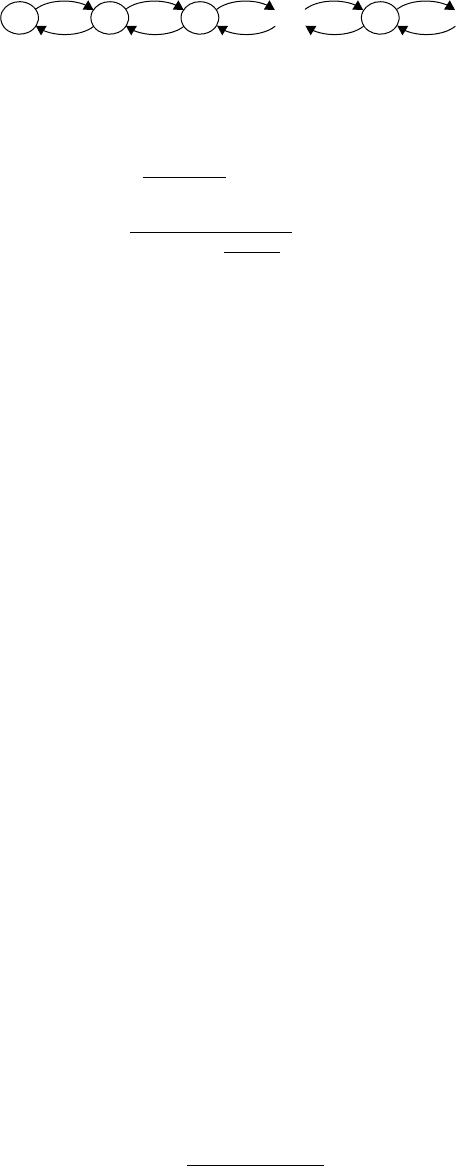
The key observation is that the state transition diagram of a simple queueing model, such as the one

in Figure 25.1, is that of a birth–death Markov chain as seen in Figure 25.3: in such a DES, there are

two events, a “birth” and a “death” with a state X(t) and an underlying state space {0, 1, ...}. The time

between births is exponentially distributed and its (generally state-dependent) birth rate parameter is λ

i =0, 1, .... Similarly, the time between deaths (deﬁned only when X(t) > 0) is exponentially distributed

and its death rate parameter is µ

, i =1, 2, .... It is easy to see that this model also represents a queueing

process where births correspond to customer arrivals and deaths correspond to customer departures.

Birth–death Markov chains have been extensively studied in the stochastic process literature. Of particular

interest for our purposes is the fact that the steady-state probabilities π

, n =0, 1, ... of such a chain are

given by (see, e.g., Cassandras and Lafortune, 1999; Kleinrock, 1975).

Queueing System Models 25-9

0 1 2 n

……

n⫺1

n⫹1

FIGURE 25.3 State transition rate diagram of a birth–death Markov chain.



···λ

n−1

···µ



, n = 1, 2, ... (25.27)

1 +



∞

n=1



···λ

n−1

···µ



(25.28)

where λ

and µ

are the birth and death rates, respectively, when the state is n.

Before proceeding with applications of this general result to Markovian queueing models, let us discuss

an important property of the Poisson process, which has signiﬁcant implications to our analysis. Looking

once again at the single-server system of Figure 25.1, consider the event [arriving customer at time t ﬁnds

X(t) =n] that is to be compared to the event [system state at some time t is X(t) =n]. The distinction

may be subtle, but it is critical. In the ﬁrst case, the observation of the system state (queue length) occurs

at speciﬁc time instants (arrivals), which depend on the nature of the arrival process. In the second case,

the observation of the system state occurs at random time instants. In general,

P[arriving customer at time t ﬁnds X(t) = n] =

P[system state at some time t is X(t) = n]

However, equality does hold for a Poisson arrival process (Kleinrock, 1975), regardless of the service time

distribution, as long as the arrival and service processes are independent. This is also known as the Poisson

Arrivals See Time Averages (PASTA) property. Using the notation π

(t) =P[system state at some time t

is X(t) =n] and α

(t) ≡P [arriving customer at time t ﬁnds X(t) =n], the PASTA property asserts that

(t) =α

(t).

Theorem 1. For a queueing system with a Poisson arrival process independent of the service process, the

probability that an arriving customer ﬁnds n customers in the system is the same as the probability that the

system state is n, i.e., π

(t) = α

(t).

Using Eq. (25.27)–(25.28) above, as well as Theorem 1, it is possible to analyze a number of Markovian

queueing systems of practical interest. We will limit ourselves here to the M/M/1 queueing system and

refer the reader to the queueing theoretic literature where more such systems are analyzed extensively

(e.g., Asmussen, 2003; Kleinrock, 1975; Trivedi, 1982).

25.6.1 The M/M/1 Queueing System

Using the notation we have established, this is a single-server system with inﬁnite storage capacity and

exponentially distributed interarrival and service times. It can therefore be modeled as a birth–death chain

with a state transition rate diagram as shown in Figure 25.3 with birth and death parameters λ

=λ for all

n =0, 1, ...and µ

=µ for all n =1, 2, ....It follows from Eq. (25.28) that

1 +



∞

n=1

(λ/µ)

25-10 Handbook of Dynamic System Modeling

The sum in the denominator is a simple geometric series that converges as long as λ/µ < 1. Under this

assumption, we get

∞



n=1





λ/µ

1 −λ/µ

and, therefore,

= 1 −

(25.29)

Letussetρ =λ/µ, which is the trafﬁc intensity deﬁned in Eq. (25.9). Thus, we see that

= 1 −ρ (25.30)

which is in agreement with Eq. (25.11). Note also that 0 ≤ρ<1, since Eq. (25.29) was derived under the

assumption λ/µ < 1.

Next, using Eq. (25.30) in Eq. (25.27), we obtain π





(1 −ρ)or

= (1 −ρ)ρ

, n = 0, 1, ... (25.31)

Eq. (25.31) gives the stationary probability distribution of the queue length of the M/M/1 system. The

condition ρ =λ/µ < 1isthestability condition for the M/M/1 system. We are now in a position to obtain

explicit expressions for various performance measures of this system.

Utilization and Throughput. The utilization is immediately given by Eq. (25.30), since 1 −π

=ρ.The

throughput is the departure rate of the server, which is µ(1 −π

) =λ. This is to be expected since at steady

state the arrival and departure rates are balanced. Thus, for a stable M/M/1 system, the throughput is

simply the arrival rate λ. In contrast, if we allow λ>µ, then the throughput is simply µ, since the server

is constantly operating at rate µ.

Average Queue Length. This is the expectation of the random variable X whose distribution is given by

Eq. (25.31). Thus,

E[X] =

∞



n=0

nπ

= (1 −ρ)

∞



n=0

nρ

(25.32)

We can evaluate the preceding sum by observing that

dρ



∞



n=0



∞



n=0

nρ

n−1

∞



n=0

nρ

Since



∞

n=0

1 −ρ

and

dρ



1 −ρ



(1 −ρ)

,weget

∞



n=0

nρ

(1 −ρ)

Then, Eq. (25.32) gives

E[X] =

1 −ρ

(25.33)

Note that as ρ →1, E[X] →∞, that is, the expected queue length grows to ∞. This clearly reveals the

tradeoff we already identiﬁed earlier: As we attempt to keep the server as busy as possible by increasing

the utilization ρ, the quality of service provided to a typical customer declines, since, on the average, such

a customer sees an increasingly longer queue length ahead of him.

Average System Time. Using Eq. (25.33) and Little’s Law in Eq. (25.24), we get

1 −ρ

= λE[S]

Queueing System Models 25-11

or, since λ =ρµ,

E[S] =

1/µ

1 −ρ

(25.34)

As ρ →0, we see that E[S] →1/µ, which is the average service time. This is to be expected, since at very

low utilizations the only delay experienced by a typical customer is a service time. We also see that as

ρ →1, E[S] →∞. Once again, this is a manifestation of the tradeoff between utilization and system time:

the higher the utilization (good for the server), the higher the average system time (bad for the customers).

Owing to the nonlinear nature of this relationship, the issue of sensitivity is crucial in queueing systems.

Our day-to-day life experience (trafﬁc jams, long ticket lines, etc.) suggests that when a queue length starts

building up, it tends to build up very fast. This is a result of operating in the range of ρ values where the

additional increase in the arrival rate causes drastic increases in E[S].

Average Waiting Time. It follows from Eqs. (25.5)–(25.6) at steady state that E[S] =E[W] +E[Z] =

E[W] +1/µ. Then, from Eq. (25.34) we get

E[W] =

1/µ

1 −ρ

−

E[W] =

µ(1 −ρ)

(25.35)

As expected, we see once again that as ρ →1, E[W] →∞, that is, increasing the system utilization toward

its maximum value leads to extremely long average waiting times for customers.

Before leaving the M/M/1 system, we brieﬂy discuss the issue of determining the transient solution

for the queue length probabilities π

(t) =P[X(t) =n], n =0, 1, .... This requires solving a set of ﬂow

balance equations obtained from Figure 25.3 with λ

=λ and µ

=µ:

dπ

(t)

=−(λ + µ)π

(t) +λπ

n−1

(t) +µπ

n+1

(t), n = 1, 2, ... (25.36)

dπ

(t)

=−λπ

(t) +µπ

(t) (25.37)

Obtaining the solution π

(t), n =0, 1, ..., of these equations is a tedious task. We provide the ﬁnal result

below to give the reader an idea of the complexity involved even for the simplest of all interesting queueing

systems we can consider (see also Asmussen, 2003; Kleinrock, 1975):

(t) = e

−(λ+µ)t

⎡

⎣

(n−i)/2

n−i

(at) +ρ

(n−i−1)/2

n+i+1

(at) +(1 − ρ)ρ

∞



j=n+i−2

−j/2

(at)

⎤

⎦

where the initial condition is π

(0) =P[X(0) =i] =1 for some given i =0, 1, ..., and a =2µρ

1/2

(x) =

∞



k=0

(x/2)

n+2k

(n +k)!k!

, n =−1, 0, 1, ...

Here, J

(x) is a modiﬁed Bessel function, which makes the evaluation of π

(t) particularly complicated.

25.7 Markovian Queueing Networks

The queueing systems we have considered thus far involve customers requesting service from a single

service-providing facility (with one or more servers). In practice, however, it is common for two or

more servers to be connected so that a customer proceeds from one server to the next in some fashion.

25-12 Handbook of Dynamic System Modeling

In communication networks, for instance, messages often go through several switching nodes followed

by transmission links before arriving at their destination. In manufacturing, a part must usually proceed

through several operations in series before it becomes a ﬁnished product. This leads to models referred to

as queueing networks, where multiple servers and queues are interconnected. In such systems, a customer

enters at some point and requests service at some server. Upon completion, the customer generally moves

to another queue or server for additional service. In the class of open networks, arriving customers from

the outside world eventually leave the system. In the class of closed networks, the number of customers

remains ﬁxed.

In the simple systems considered thus far, our objective was to obtain the stationary probability dis-

tribution of the state X,whereX is the queue length. In networks, we have a system consisting of M

interconnected nodes, where the term “node” is used to describe a set of identical parallel servers along

with the queueing space that precedes it. In a network environment, we shall refer to X

as the queue length

at the ith node in the system, i =1, ... , M. It follows that the state of a Markovian queueing network is a

vector of random variables

X = [X

, X

, ... , X

] (25.38)

where X

takes on values n

=0, 1, ... just like a simple single-class stand-alone queueing system. The

major objective of queueing network analysis is to obtain the stationary probability distribution of X (if it

exists), i.e., the probabilities

π(n

, ... , n

) = P[X

= n

, ... , X

= n

] (25.39)

for all possible values of n

, ... , n

, n

=0, 1, ....

In the next few sections, we present the main results pertinent to the analysis of Markovian queueing

networks. This means that all external arrival events and all departure events at the servers in the system are

generated by processes satisfying the Markovian (memoryless) property, and are therefore characterized

by exponential distributions. A natural question that arises is: “what about internal arrival processes?” In

other words,the arrival process at some queue in the network is usually composed of one or more departure

processes from adjacent servers; what are the stochastic characteristics of such processes? The answer to

this question is important for much of the classical analysis of queueing networks and is presented in the

next section.

25.7.1 The Departure Process of the M/M/1 Queueing System

Let us consider an M/M/1 queueing system. Recall that Y

and Z

denote the interarrival and service time,

respectively, of the kth customer, and that the arrival and service processes are assumed to be independent.

Now let us concentrate on the departure times D

, k =1, 2, ..., of customers, and deﬁne 

to be the

kth interdeparture time, that is, a random variable such that 

−D

k−1

is the time elapsed between

the (k −1)th and the kth departure, k =1, 2, ..., where, for simplicity, we set 

=0, so that 

is the

random variable describing the time of the ﬁrst departure. As k →∞, we will assume that there exists a

stationary probability distribution function such that

lim

k→∞

P[

≤ t] = P[ ≤ t]

where  describes an interdeparture time at steady state. We will now evaluate the distribution P[ ≤t].

The result, stated below as a theorem without proof (see also Buzen, 1973) is quite surprising:

Theorem 2. The departure process of a stable stationary M/M/1 queueing system with arrival rate λ is a

Poisson process with rate λ, i.e., P[ ≤t] =1 −e

−λt

This fundamental property of the M/M/1 queueing system is also known as Burke’s theorem (Burke,

1956): a Poisson process supplying arrivals to a server with exponentially distributed service times results

Queueing System Models 25-13

in a Poisson departure process with the exact same rate. This fact also holds for the departure process

of an M/M/m system. Burke’s theorem has some critical ramiﬁcations when dealing with networks of

Markovian queueing systems, because it allows us to treat each component node independently, as long

as there are no customer feedback paths. When a node is analyzed independently, the only information

required is the number of servers at that node, their service rate, and the arrival rate of customers (from

other nodes as well as the outside world).

25.7.2 Open Queueing Networks

We will consider a general open network model consisting of M nodes, each with inﬁnite storage capacity.

We willassume that customers form a single class, and that all nodes operate accordingto an FCFS queueing

discipline. Node i, i =1, ... , M, consists of m

servers each with exponentially distributed service times

with parameter µ

. External customers may arrive at node i from the outside world according to a Poisson

process with rate r

. In addition, internal customers arrive from other servers in the network. Upon

completing service at node i, a customer is routed to node j with probability p

; this is referred to as the

routing probability from i to j. The outside world is usually indexed by 0, so that the fraction of customers

leaving the network after service at node i is denoted by p

. Note that p

=1 −



j=1

In this modeling framework, let λ

denote the total arrival rate at node i. Thus, using the notation above,

we have

= r



j=1

, i = 1, ..., M (25.40)

where the ﬁrst term represents the external customer ﬂow and the second term represents the aggregate

internal customer ﬂow from all other nodes.

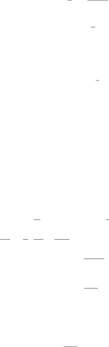
Before discussing the general model, let us ﬁrst consider the simplest possible case, consisting of two

single-server nodes in tandem, as shown in Figure 25.4. In this case, the state of the system is the two-

dimensional vector X =[X

, X

], where X

, i =1, 2, is the queue length of the ith node. Since all events are

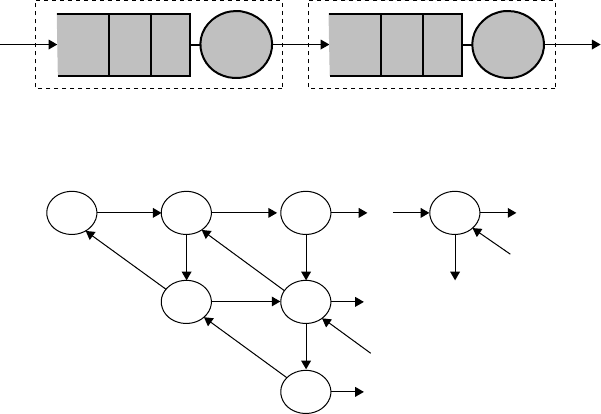
generated by Poisson processes, we can model the system as a Markov chain whose state transition rate

diagram is shown in Figure 25.5.

␭

␮

FIGURE 25.4 A two-node open queueing network. (From Cassandras, C.G., and Lafortune, S., Introduction to

Discrete Event Systems, Springer, Berlin, 1999, pp. 485–486.)

0,0 1,0

0,1 1,1

0,1

2,0 n

…

␭␭

␭

␮

FIGURE 25.5 State transition rate diagram for a two-node open queueing network. (From Cassandras, C.G., and

Lafortune, S., Introduction to Discrete Event Systems, Springer, Berlin, 1999, pp. 485–486.)