Farin G. Curves and Surfaces for CAGD. A Practical Guide
Подождите немного. Документ загружается.

382 Chapter 21 Surfaces with Arbitrary Topology
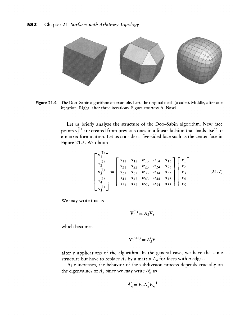
Figure 21.4 The Doo-Sabin algorithm: an example. Left, the original mesh (a
cube).
Middle, after one
iteration. Right, after three iterations. Figure courtesy A. Nasri.
Let us briefly analyze the structure of the Doo-Sabin algorithm. New face
points
V-
are created from previous ones in a linear fashion that lends itself to
a matrix formulation. Let us consider a five-sided face such as the center face in
Figure 21.3. We obtain
rvf^i
vf
r^'
U?
V.f\
=
0^11 «12 ^13 (^U ^\S
«21 «22 «23 0^24 «25
«31 «32 «33 «34 «35
«41 «42 «43 «44 «45
.0^51 «52 «53 <^54 «55 J
V2
V3
V4
LV5.
(21.7)
We may write this as
which becomes
N^^^=As\,
V(^+1)^A;V
after r applications of the algorithm. In the general case, we have the same
structure but have to replace A5 by a matrix A„ for faces with n edges.
As r increases, the behavior of the subdivision process depends crucially on
the eigenvalues of A„ since we may write A^ as
^^ -
^n^'^n^n
-1
21.3 CatmuU-Clark Subdivision 383
following the approach of Section 21.1. Since all rows of A„ sum to unity, one
eigenvalue is Xi = 1. The remaining ones are all real since A is symmetric and
are all between 0 and 1 since each V^^ is contained in the convex hull of V^^~^\
An exact analysis of this process is fairly involved and is omitted here. It reveals,
however, that Doo-Sabin surfaces are G^ everywhere. For more details, see [174]
or [18], [19],
[503].
The matrices A„ are circularity and their eigenstructure has
been studied in detail by
P.
Davis
[134].
A matrix is circulant if each row may be
obtained from the previous row by a "right shift."
Figure 21.4 gives an example of several steps of the algorithm.
As a rather trivial observation, Doo-Sabin surfaces have the convex hull and
local control properties, and their construction is affinely invariant. But they also
do not need an underlying parametrization, which makes them more geometric
than tensor product B-spline surfaces. A drawback of this nice feature is the
problem of point evaluation: though we can evaluate as many points as close to
the surface as we like, computation of just one point is not trivial.
One set of points on the surface is easy to identify: at every level of subdivision,
the centroid of any face will be on the final surface. For a
proof,
we observe that
any face will produce a sequence of F-faces converging to its centroid. In the
limit, the centroid is thus on the surface.
21.5 Catmull-Clark Subdivision
The same issue of Computer-Aided Design that included the Doo-Sabin al-
gorithm also contained a competing method, invented by E. CatmuU and J.
Clark; see
[103].
Whereas Doo-Sabin surfaces are a generalization of biquadratic
B-splines to arbitrary topology, Catmull-Clark surfaces generalize bicubic
B-spline surfaces to arbitrary topology.
We start with a polygonal mesh MP consisting of vertices v9. We iteratively
refine the mesh, resulting in finer and finer meshes M\ consisting of vertices v^.
Each refinement step can be described by explaining what happens locally for
the points adjacent to a vertex v^:
1.
Form face points f ^^: for each face in the mesh, find the centroid of its
vertices.
2.
Form edge points e-^ : for each edge in the mesh, average the edge's
endpoints and the two face points on either side of the edge.
3.
Form a new vertex point v^"^^: assuming there are n faces around v^, it is
computed as follows:
384 Chapter 21 Surfaces with Arbitrary Topology
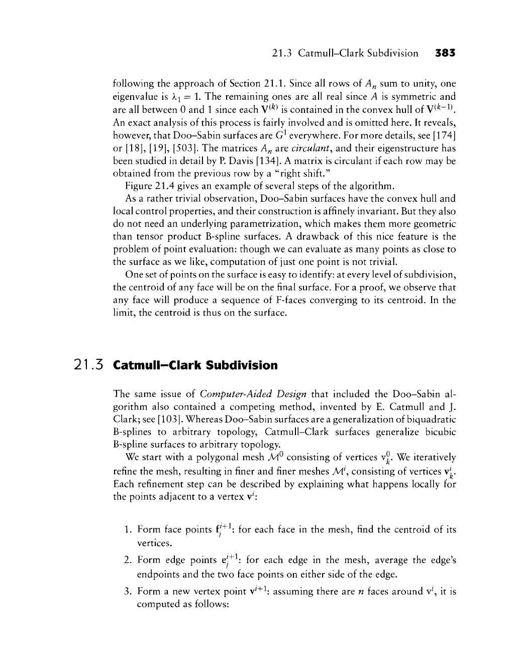
Figure 21.5 The Catmull-Clark algorithm: the original control net (black) and one level of subdivision
(gray).
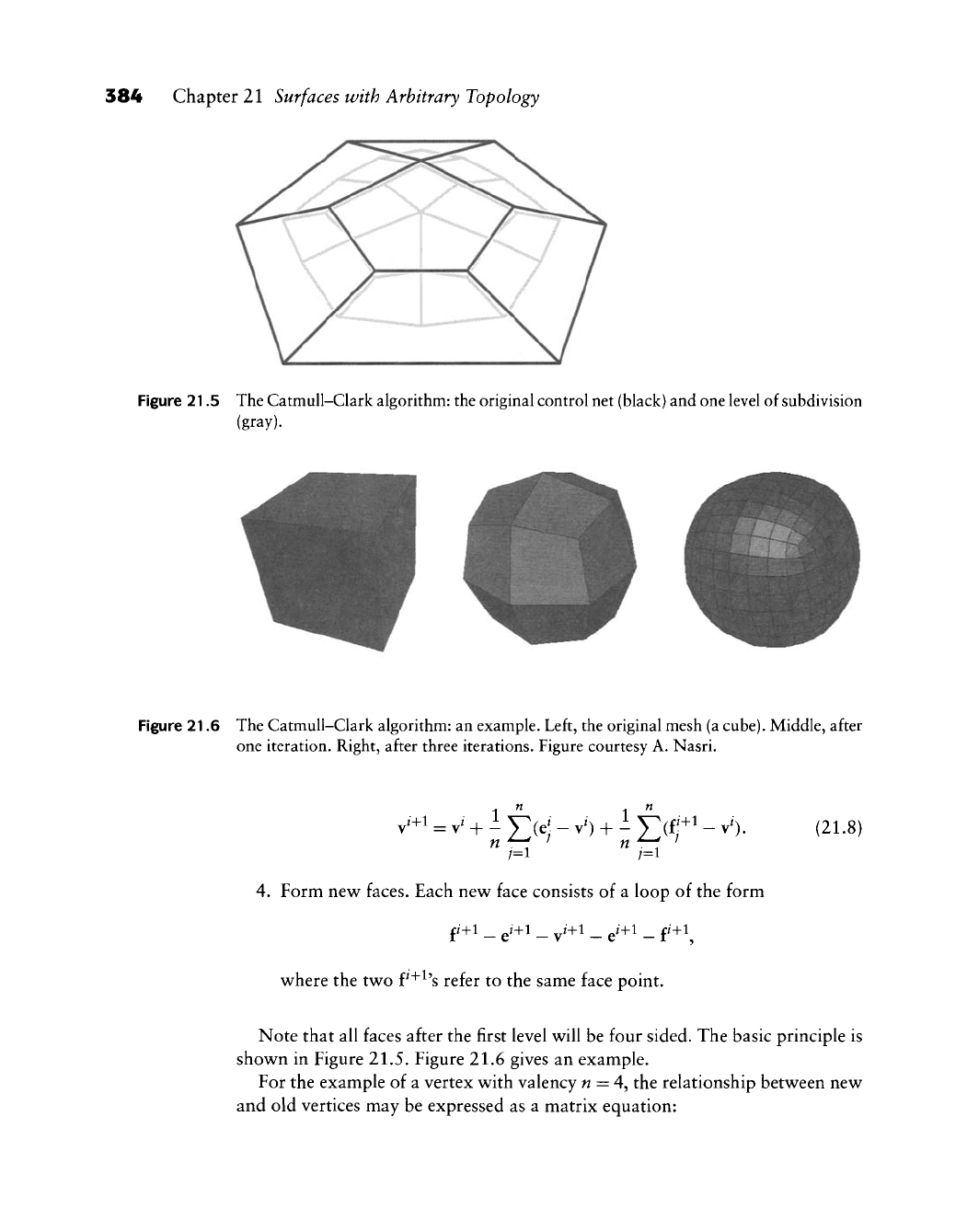
Figure 21.6 The Catmull-Clark algorithm: an example. Left, the original mesh (a
cube).
Middle, after
one iteration. Right, after three iterations. Figure courtesy A. Nasri.
J+^
- J
;=i
"7=1
(21.8)
4.
Form new faces. Each nev^ face consists of a loop of the form
where the two P"^^'s refer to the same face point.
Note that all faces after the first level will be four sided. The basic principle is
shown in Figure 21.5. Figure 21.6 gives an example.
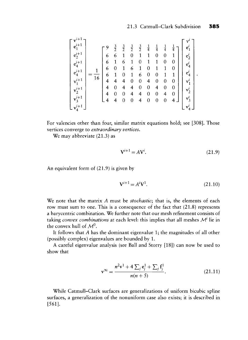
For the example of a vertex with valency
w
= 4, the relationship between new
and old vertices may be expressed as a matrix equation:
21.3 CatmuU-Clark Subdivision 385
J_
16
9
6
6
6
6
4
4
4
4
3
6
1
0
1
4
0
0
4
3
2
1
6
1
0
4
4
0
0
3
2
0
1
6
1
0
4
4
0
3
2
1
0
1
6
0
0
4
4
1
4
1
1
0
0
4
0
0
0
1
4
0
1
1
0
0
4
0
0
1
4
0
0
1
1
0
0
4
0
1
4
1
0
0
1
0
0
0
4
V
For valencies other than four, similar matrix equations hold; see
[308].
Those
vertices converge to extraordinary vertices.
We may abbreviate (21.3) as
7'+l .
:AV'. (21.9)
An equivalent form of (21.9) is given by
V+i = A^Vi.
(21.10)
We note that the matrix A must be stochastic^ that is, the elements of each
row must sum to one. This is a consequence of the fact that (21.8) represents
a barycentric combination. We further note that our mesh refinement consists of
taking convex combinations at each level: this implies that all meshes M^ lie in
the convex hull of M^.
It follows that A has the dominant eigenvalue 1; the magnitudes of all other
(possibly complex) eigenvalues are bounded by 1.
A careful eigenvalue analysis (see Ball and Storry [18]) can now be used to
show that
«V + 4X:;e/ + E;f/
n{n + 5)
(21.11)
While Catmull-Clark surfaces are generalizations of uniform bicubic spline
surfaces, a generalization of the nonuniform case also exists; it is described in
[561].
386 Chapter 21 Surfaces with Arbitrary Topology
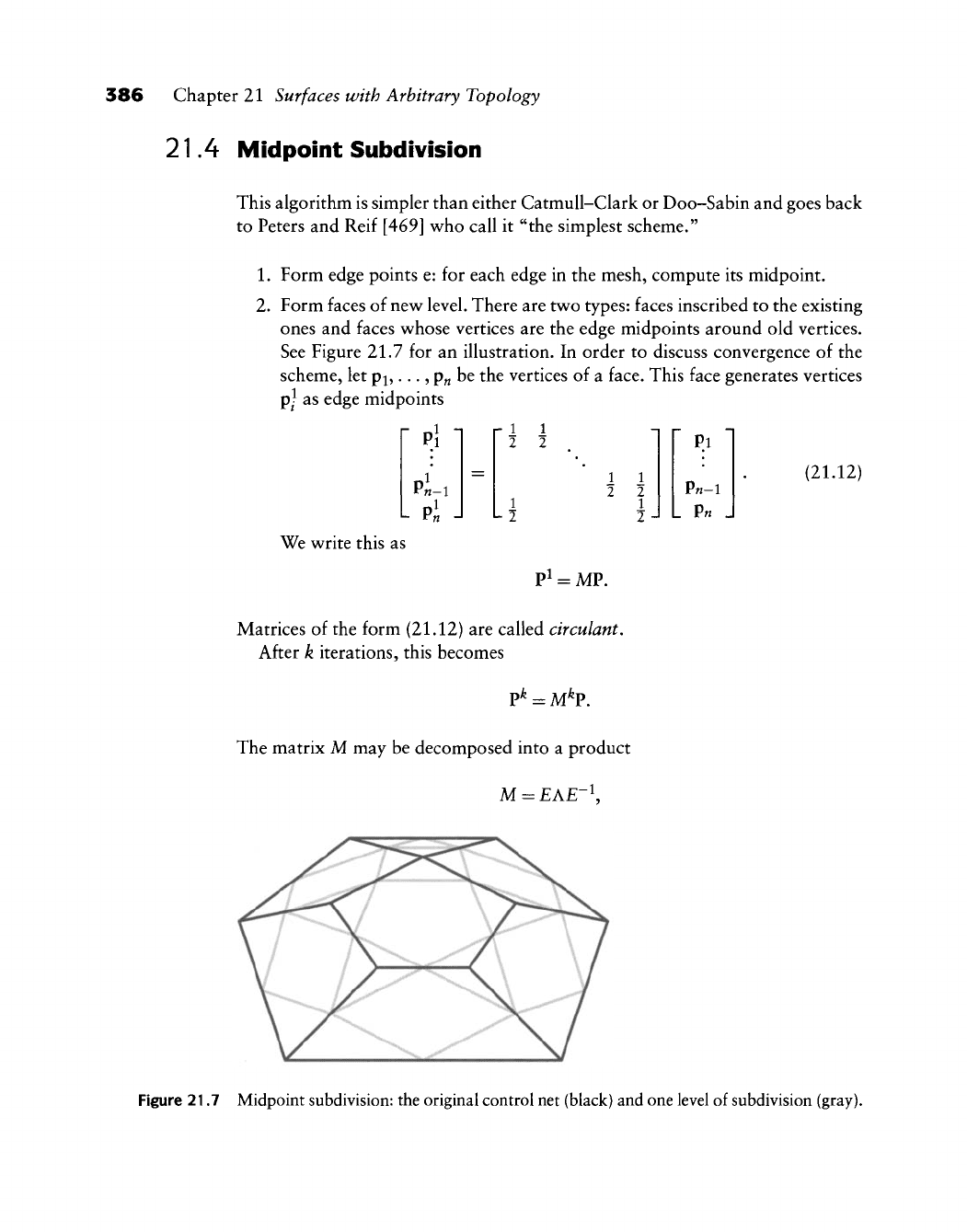
21.4 Midpoint Subdivision
This algorithm is simpler than either Catmull-Clark or Doo-Sabin and goes back
to Peters and Reif [469] who call it "the simplest scheme."
1.
Form edge points e: for each edge in the mesh, compute its midpoint.
2.
Form faces of new level. There are two types: faces inscribed to the existing
ones and faces whose vertices are the edge midpoints around old vertices.
See Figure 21.7 for an illustration. In order to discuss convergence of the
scheme, let Pi,. •., p« be the vertices of a face. This face generates vertices
p^^
as edge midpoints
["^ 1
r 1
2
1
write this as
1
2
Pl
,
1
2
= MP.
~
1
2
1
2
-J
p.l
p«-l
L P« ,
(21.12)
Matrices of the form (21.12) are called circulant.
After k iterations, this becomes
P*
= M^P.
The matrix M may be decomposed into a product
M = £A£-^
Figure 21.7 Midpoint subdivision: the original control net (black) and one level of subdivision (gray).
21.5 Loop Subdivision 387
where E is the matrix containing M's eigenvectors and A is the diagonal matrix
containing M's eigenvalues. We then have, foUov^ing the reasoning in Section
21.1,
M^ = £A^£-K
The analysis of the limit process is thus closely related to the eigenstructure of
M. A result from Davis [134] asserts that for any initial polygon P, we obtain
regular planar polygons in the limit. These will be the tangent planes to our
surface, which therefore is G^
21.5 Loop Subdivision
A triangle-based subdivision scheme was discussed by C. Loop
[397].
Its input
is a triangular mesh as discussed in Section 21.9. It then successively refines this
mesh, resulting in a smooth limit surface.
Loop subdivision proceeds as follows.
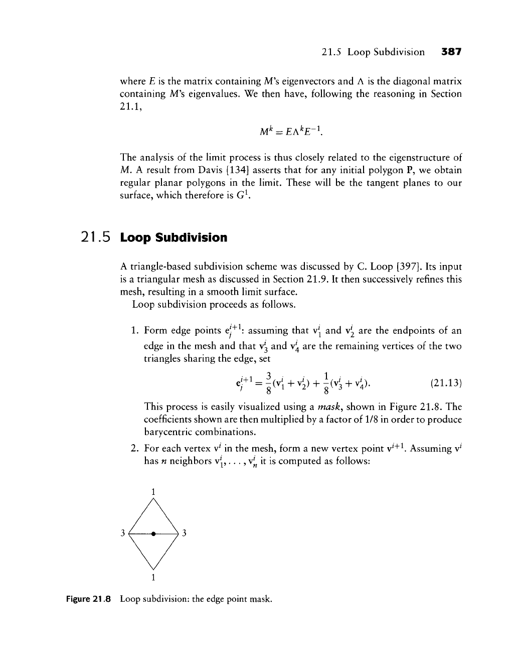
1.
Form edge points ej"^ : assuming that v^^ and Vj are the endpoints of an
edge in the mesh and that v^ and v^ are the remaining vertices of the two
triangles sharing the edge, set
^r'=^K+^1)+^(^3+<)• (21-13)
This process is easily visualized using a masky shown in Figure 21.8. The
coefficients shown are then multiplied by a factor of 1/8 in order to produce
barycentric combinations.
2.
For each vertex
v^
in the mesh, form a new vertex point v^"^^ Assuming v^
has n neighbors v^ . . ., v^ it is computed as follows:
1
Figure 21.8 Loop subdivision: the edge point mask.
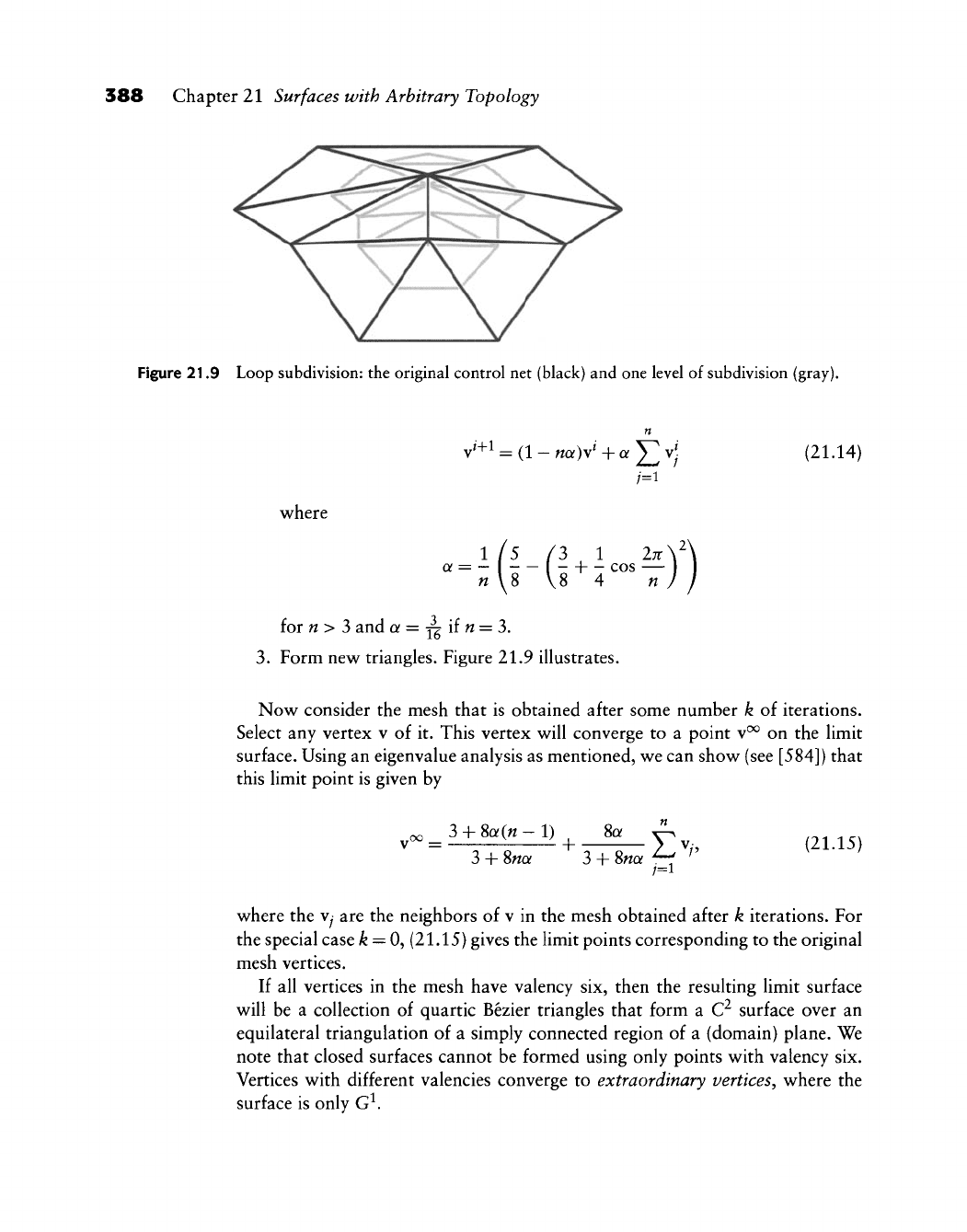
388 Chapter 21 Surfaces with Arbitrary Topology
Figure 21.9 Loop subdivision: the original control net (black) and one level of subdivision (gray).
v^+1
=
(1
- naW + « 1] ^/ (21.14)
where
1/5 /3 1 27r\^\
a = - \ - + - cos —
« \8 V8 4 n ) I
for n> 3 and a =
j^iin
=
?>.
3.
Form new triangles. Figure 21.9 illustrates.
Now consider the mesh that is obtained after some number k of iterations.
Select any vertex v of it. This vertex will converge to a point v^ on the limit
surface. Using an eigenvalue analysis as mentioned, we can show (see [584]) that
this limit point is given by
3 + 8(y(fz-l)
3 + 8wa
+
8a
3
+ 8«a
/=1
(21.15)
where the
Vy
are the neighbors of v in the mesh obtained after k iterations. For
the special case ^ = 0, (21.15) gives the limit points corresponding to the original
mesh vertices.
If all vertices in the mesh have valency six, then the resulting limit surface
will be a collection of quartic Bezier triangles that form a C^ surface over an
equilateral triangulation of a simply connected region of a (domain) plane. We
note that closed surfaces cannot be formed using only points with valency six.
Vertices with different valencies converge to extraordinary vertices^ where the
surface is only G^.
21.7 Interpolating Subdivision Surfaces 389
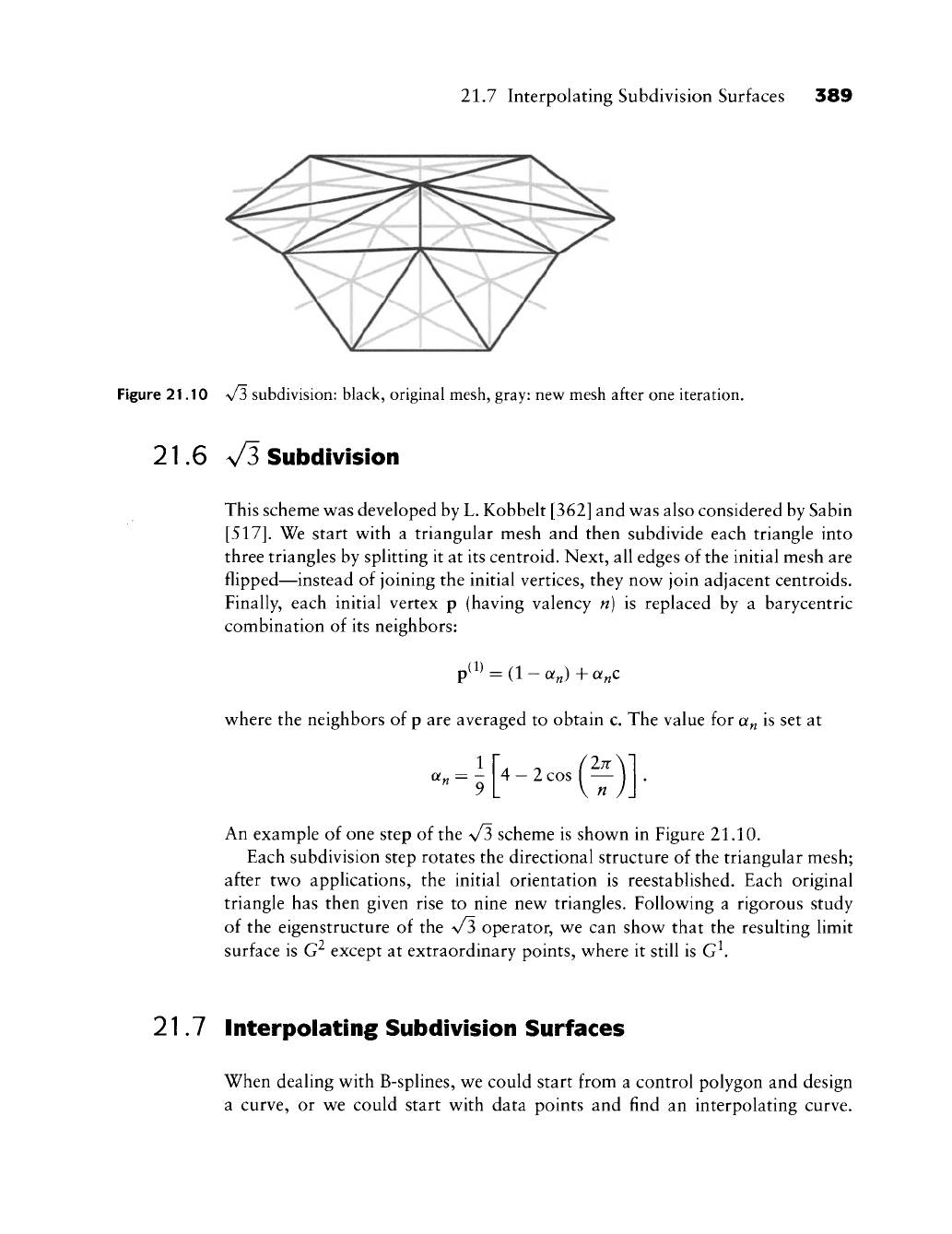
Figure 21.10 \/3 subdivision: black, original mesh, gray: new mesh after one iteration.
21.6 V3 Subdivision
This scheme was developed by L. Kobbelt [362] and was also considered by Sabin
[517].
We start with a triangular mesh and then subdivide each triangle into
three triangles by splitting it at its centroid. Next, all edges of the initial mesh are
flipped—instead of joining the initial vertices, they now join adjacent centroids.
Finally, each initial vertex p (having valency n) is replaced by a barycentric
combination of its neighbors:
.(1)
p^'^
= (1 - a J +
a„c
where the neighbors of p are averaged to obtain c. The value for a^ is set at
1
^ 9
4_2cos(—")
An example of one step of the \/3 scheme is shown in Figure 21.10.
Each subdivision step rotates the directional structure of the triangular mesh;
after two applications, the initial orientation is reestabUshed. Each original
triangle has then given rise to nine new triangles. Following a rigorous study
of the eigenstructure of the \/3 operator, we can show that the resulting limit
surface is G^ except at extraordinary points, where it still is G^.
21.7 interpolating Subdivision Surfaces
When dealing with B-splines, we could start from a control polygon and design
a curve, or we could start with data points and find an interpolating curve.
390 Chapter 21 Surfaces with Arbitrary Topology
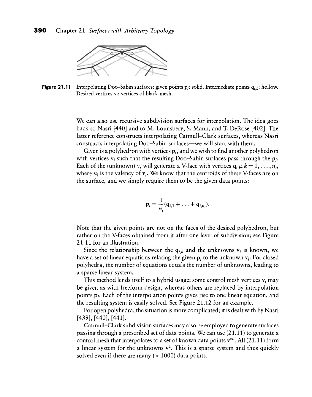
Figure 21.11 Interpolating Doo-Sabin surfaces: given points
p^:
solid. Intermediate points
q^^^:
hollow.
Desired vertices
v^:
vertices of black mesh.
We can also use recursive subdivision surfaces for interpolation. The idea goes
back to Nasri [440] and to M. Lounsbery, S. Mann, and T. DeRose
[402].
The
latter reference constructs interpolating Catmull-Clark surfaces, w^hereas Nasri
constructs interpolating Doo-Sabin surfaces—v^e will start w^ith them.
Given is a polyhedron with vertices
p^,
and we wish to find another polyhedron
with vertices V/ such that the resulting Doo-Sabin surfaces pass through the p^.
Each of the (unknown) v^ will generate a V-face with vertices q^^; ^ = 1,. ..,
w^,
where fii is the valency of
v^.
We know that the centroids of these V-faces are on
the surface, and we simply require them to be the given data points:
1
fl:
'
Note that the given points are not on the faces of the desired polyhedron, but
rather on the V-faces obtained from it after one level of subdivision; see Figure
21.11 for an illustration.
Since the relationship between the
q^
^^
and the unknowns v^ is known, we
have a set of linear equations relating the given
p^
to the unknown v^. For closed
polyhedra, the number of equations equals the number of unknowns, leading to
a sparse linear system.
This method lends itself to a hybrid usage: some control mesh vertices v/ may
be given as with freeform design, whereas others are replaced by interpolation
points p/. Each of the interpolation points gives rise to one linear equation, and
the resulting system is easily solved. See Figure 21.12 for an example.
For open polyhedra, the situation is more complicated; it is dealt with by Nasri
[439], [440], [441].
CatmuU-Clark subdivision surfaces may also be employed to generate surfaces
passing through a prescribed set of data points. We can use (21.11) to generate a
control mesh that interpolates to a set of known data points v^. All (21.11) form
a linear system for the unknowns v^. This is a sparse system and thus quickly
solved even if there are many (> 1000) data points.
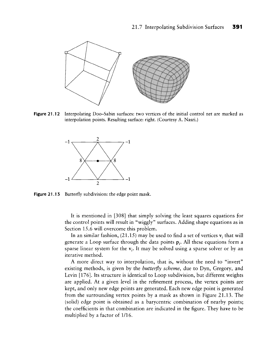
21.7 Interpolating Subdivision Surfaces 391
Figure 21.12 Interpolating Doo-Sabin surfaces: two vertices of the initial control net are marked as
interpolation points. Resulting surface: right. (Courtesy A. Nasri.)
Figure 21.13 Butterfly subdivision: the edge point mask.
It is mentioned in [308] that simply solving the least squares equations for
the control points will result in "wiggly" surfaces. Adding shape equations as in
Section 15.6 will overcome this problem.
In an similar fashion, (21.15) may be used to find a set of vertices v^ that will
generate a Loop surface through the data points p^. All these equations form a
sparse linear system for the V/. It may be solved using a sparse solver or by an
iterative method.
A more direct way to interpolation, that is, without the need to "invert"
existing methods, is given by the butterfly scheme^ due to Dyn, Gregory, and
Levin
[176].
Its structure is identical to Loop subdivision, but different weights
are applied. At a given level in the refinement process, the vertex points are
kept, and only new edge points are generated. Each new edge point is generated
from the surrounding vertex points by a mask as shown in Figure
21.13.
The
(solid) edge point is obtained as a barycentric combination of nearby points;
the coefficients in that combination are indicated in the figure. They have to be
multiplied by a factor of 1/16.