Farin G. Curves and Surfaces for CAGD. A Practical Guide
Подождите немного. Документ загружается.

112 Chapter 7 Polynomial Curve Constructions
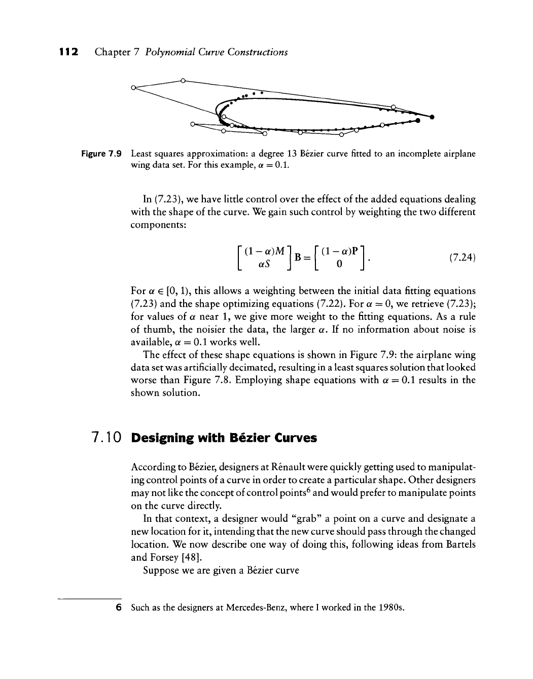
Figure 7.9 Least squares approximation: a degree 13 Bezier curve fitted to an incomplete airplane
wing data set. For this example, a = 0.1.
In (7.23), we have little control over the effect of the added equations deahng
with the shape of the curve. We gain such control by weighting the two different
components:
[";r]-["Tl-
(7.24)
For a e [0,1), this allows a weighting between the initial data fitting equations
(7.23) and the shape optimizing equations (7.22). For a = 0, we retrieve (7.23);
for values of a near 1, we give more weight to the fitting equations. As a rule
of thumb, the noisier the data, the larger a. If no information about noise is
available, a = 0.1 works well.
The effect of these shape equations is shown in Figure 7.9: the airplane wing
data set was artificially decimated, resulting in a least squares solution that looked
worse than Figure 7.8. Employing shape equations with a = 0.1 results in the
shown solution.
7.10 Designing witii Bezier Curves
According to Bezier, designers at Renault were quickly getting used to manipulat-
ing control points of a curve in order to create a particular shape. Other designers
may not like the concept of control points^ and would prefer to manipulate points
on the curve directly.
In that context, a designer would "grab" a point on a curve and designate a
new location for it, intending that the new curve should pass through the changed
location. We now describe one way of doing this, following ideas from Barrels
and Forsey [48].
Suppose we are given a Bezier curve
6 Such as the designers at Mercedes-Benz, where I worked in the 1980s.
7.10 Designing with Bezier Curves 113
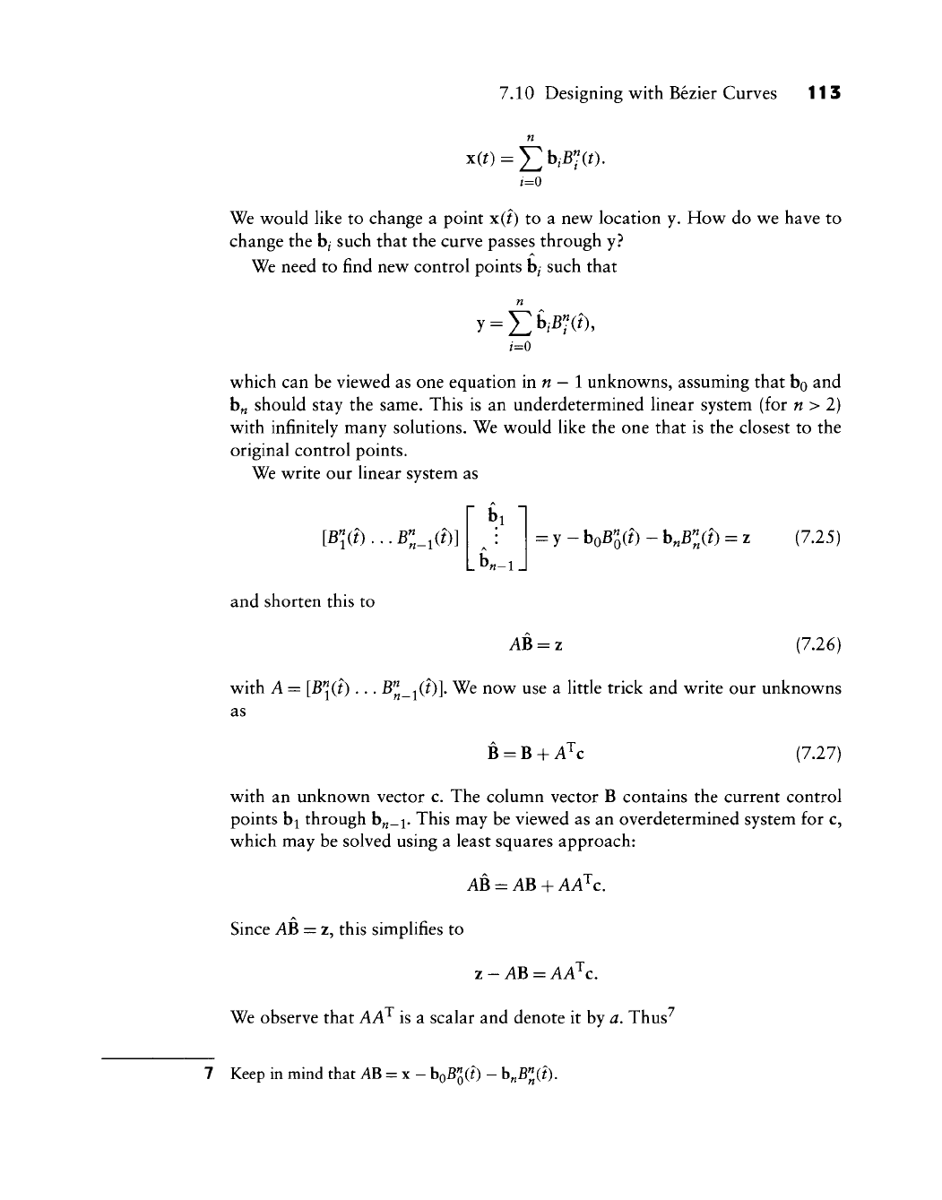
n
i=0
We would like to change a point x{i) to a new location y. How do we have to
change the b/ such that the curve passes through y?
We need to find new control points b/ such that
y
=
X]W^^
i=0
which can be viewed as one equation inn— 1 unknowns, assuming that bo and
b„ should stay the same. This is an underdetermined linear system (for n > 2)
with infinitely many solutions. We would like the one that is the closest to the
original control points.
We write our linear system as
[B",ii)...B"„_,ii)]
and shorten this to
Lb«-i J
= y-boB^(?)-b,B^(?) = z (7.25)
AB = z (7.26)
with A = [B^(i)...
B^_-^(i)],
We now use a little trick and write our unknowns
as
B = B + A^c (7.27)
with an unknown vector c. The column vector B contains the current control
points bi through b„_i. This may be viewed as an overdetermined system for c,
which may be solved using a least squares approach:
AB = AB + AA'^C.
Since AB = z, this simplifies to
z - AB = AA'^C.
We observe that AA^ is a scalar and denote it by a. Thus'^
7 Keep in mind that
AB
= x - hoB^ii) - b„B^(?).
114 Chapter 7 Polynomial Curve Constructions
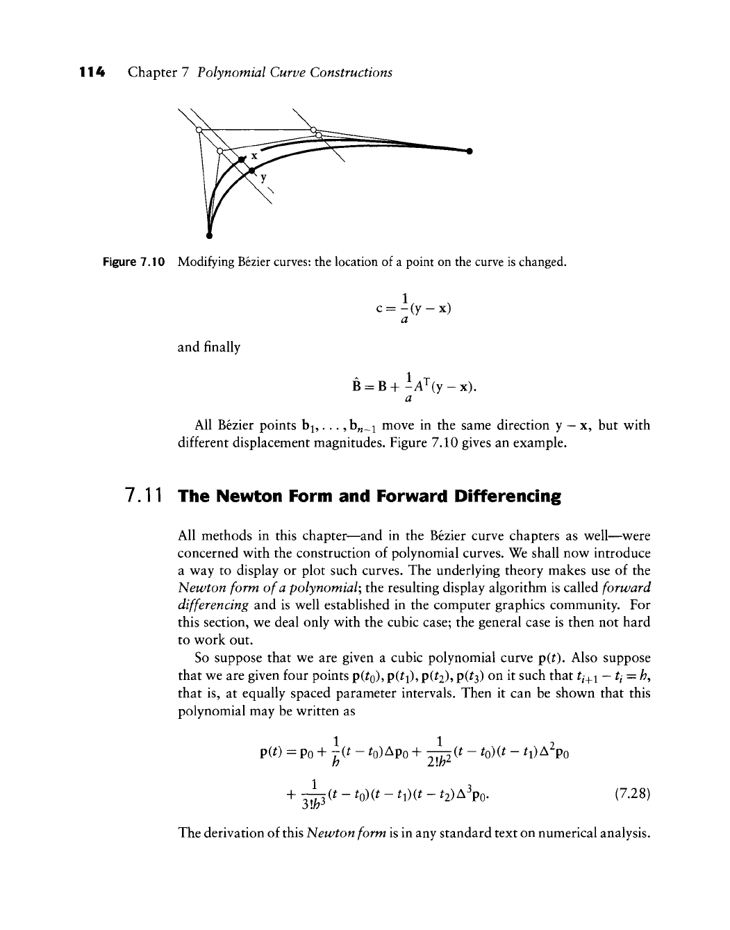
Figure 7.10 Modifying Bezier curves: the location of a point on the curve is changed.
and finally
c=-(y-x)
a
B = B+-A'^(y-x).
All Bezier points b^,. .., b„_i move in the same direction y
—
x, but v^ith
different displacement magnitudes. Figure 7.10 gives an example.
7.11 The Newton Form and Forward Differencing
AH methods in this chapter—and in the Bezier curve chapters as well—^were
concerned with the construction of polynomial curves. We shall now introduce
a way to display or plot such curves. The underlying theory makes use of the
Newton form of a polynomial; the resulting display algorithm is called forward
differencing and is well established in the computer graphics community. For
this section, we deal only with the cubic case; the general case is then not hard
to work out.
So suppose that we are given a cubic polynomial curve p(^). Also suppose
that we are given four points
pC^o)?
P(^i)?
p(h)'>
p(h) ^^ i^ such that tj^i
—
tj = h,
that is, at equally spaced parameter intervals. Then it can be shown that this
polynomial may be written as
1 1
P(^) =
Po
+ ^(* - ^o)Apo + ^it - to)it - ti)A^Po
1
(7.28)
The derivation of this Newton form is in any standard text on numerical analysis.
7.11 The Newton Form and Forward Differencing 115
The differences A^py are defined as
A'p,.
= A'-V/+i-A'-ipy (7.29)
and A^py = py.
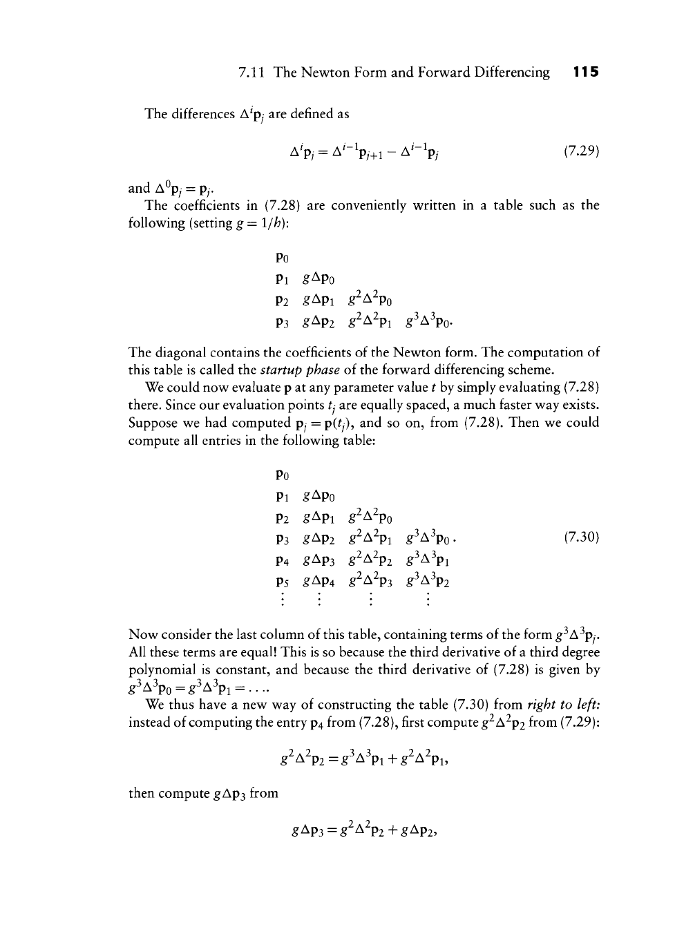
The coefficients in (7.28) are conveniently written in a table such as the
following (setting g = 1/h):
Po
Pi gApo
P2 g^Pl g^^^Po
P3 g^Pl g^^^Pl g^^W
The diagonal contains the coefficients of the Newton form. The computation of
this table is called the startup phase of the forward differencing scheme.
We could now evaluate p at any parameter value t by simply evaluating (7.28)
there. Since our evaluation points tj are equally spaced, a much faster way exists.
Suppose we had computed py = p(^y), and so on, from (7.28). Then we could
compute all entries in the following table:
Po
Pi gApo
P2 g^Pi g^A^po
P3 g^Pi g^^^Pi g^^^PO' (7-30)
P4 gAp3 g^A2p2 g^A^pi
P5 ^Ap4 g^A2p3 g^A^p2
Now consider the last column of this table, containing terms of the form g^A^py.
All these terms are equal! This is so because the third derivative of a third degree
polynomial is constant, and because the third derivative of (7.28) is given by
g^A^P0 = g^A^Pl = ....
We thus have a new way of constructing the table (7.30) from right to left:
instead of computing the entry p4 from (7.28), first compute g'^ A^p2 from (7.29):
g^A^P2=g^A^Pl+g^A^Pl,
then compute gAp3 from
gAp3 = g^A^P2+gAp2,
116 Chapter 7 Polynomial Curve Constructions
and finally
P4=gAp3 + P3.
Then compute P5 in the same manner, and so on. The general formula is, with
qj = g^A^Py:
q; = q;:^l + q;_i; / = 2,1,0. (7.31)
It yields the points py = q^^.^
This way of computing the py does not involve a single multiplication after
the startup phase! It is therefore extremely fast and has been implemented in
many graphics systems. Given four initial points po, pi, p2,
P3
and a stepsize
/?,
it
generates a sequence of points on the cubic polynomial through the initial four
points. Typically, the polynomial will be given in Bezier form, so those four points
have to be computed as a startup operation.
In a graphics environment, it is desirable to adjust the stepsize h such that
each pixel along the curve is hit. One way of doing this is to adjust the stepsize
while marching along the curve. This is called adaptive forward differencing and
is described by Lien, Shantz, and Pratt [389] and by Chang, Shantz, and Rochetti
[109].
Although fast, forward differencing is not
foolproof.
As we compute more
and more points on the curve, they begin to be affected by
roundoff.
So while we
intend to march along our curve, we may instead leave its path, deviating from it
more and more as we continue. For more literature on this method, see Abi-Ezzi
[1],
Bartels, Beatty, and Barsky [47], or Shantz and Chang
[571].
7.12 Implementation
The code for Aitken's algorithm is very similar to that for the de Casteljau
algorithm. Here is its header:
float aitken(degree,coeff,t)
/* uses Aitken to compute one coordinate
value of a Lagrange interpolating polynomial. Has to be called
for each coordinate (x,y, and/or z) of data points.
Input: degree: degree of curve.
8 It holds for any degree n if we replace / = 2,1,0 by / = «
—
1,
w —
2,...,
0.
7.13 Problems 117
coeff: array with coordinates
to be
interpolated,
t: parameter value.
Output: coordinate value.
Note:
we
assume
a
uniform knot sequence!
V
7.15 Problems
1 Show that the cubic and quintic Hermite polynomials are linearly indepen-
dent.
2 Generahze Hermite interpolation to degrees 7, 9, and so on.
* 3 The de Casteljau algorithm for Bezier curves has as its "counterpart" the
recursion formula (5.2) for Bernstein polynomials. Deduce a recursion
formula for Lagrange polynomials from Aitken's algorithm.
* 4 The de Casteljau algorithm may be generalized to yield the concept of
blossoms. This is not possible for Aitken's algorithm. Why?
* 5 The Hermite form is not invariant under affine domain transformations,
v^hereas the Bezier form
is.
What about the Lagrange and monomial forms?
What are the general conditions for a curve scheme to be invariant under
affine domain transformations?
* 6 When P = n in least squares approximation, we should be back in an
interpolation context. Shov^ that this is indeed the case.
PI Aitken's algorithm looks very similar to the de Casteljau algorithm. Use
both to define a whole class of algorithms, of which each would be a special
case (see [205]). Write a program that uses as input a parameter specifying
if the output curve should be "more Bezier" or "more Lagrange."
P2 The function that was used by Runge to demonstrate the effect that now
bears his name is given by
fW = 7^; xG[-l,l].
Use the routine ait ken to interpolate at equidistant parameter intervals.
Keep increasing the degree of the interpolating polynomial until you notice
"bad" behavior on the part of the interpolant.
P3 In Lagrange interpolation, each p^ is assigned a corresponding parameter
value tj. Experiment (graphically) by interchanging two parameter values
ti and tj without interchanging
p^
and py. Explain your results.

This Page Intentionally Left Blank
B-Spline Curves
D-splines were investigated as early as the nineteenth century by N. Lobachevsky
(see Renyi
[506],
p. 165); they were constructed as convolutions of certain prob-
ability distributions.^ In
1946,1.
J. Schoenberg [542] used B-splines for statistical
data smoothing, and his paper started the modern theory of spline approxima-
tion. For the purposes of this book, the discovery of the recurrence relations
for B-splines by C. de Boor
[137],
M. Cox
[129],
and L. Mansfield was one of
the most important developments in this theory. The recurrence relations were
first used by Gordon and Riesenfeld [284] in the context of parametric B-spline
curves.
This chapter presents a theory for arbitrary degree B-spline curves. The orig-
inal development of these curves makes use of divided differences and is math-
ematically involved and numerically unstable; see de Boor [138] or Schumaker
[546].
A different approach to B-splines was taken by de Boor and Hollig
[143];
they used the recurrence relations for B-splines as the starting point for the the-
ory. In this chapter, the theory of B-splines is based on an even more fundamental
concept: the blossoming method proposed by L. Ramshaw [498] and, in a
dif-
ferent form, by R de Casteljau
[147].
More literature on blossoms: Gallier
[252],
Boehm and Prautzsch [87].
1 However, those were only defined over a very special knot sequence.
119
120 Chapter 8 B-Spline Curves
8.1 Motivation
B-spline curves consist of many polynomial pieces, offering much more versatility
than do Bezier curves. Many B-spline curve properties can be understood by
considering just one polynomial piece—that is how
w^e
start this chapter.
The Bezier points of a quadratic Bezier curve may be written as blossom values
b[0,0],b[0,l],b[l,l].
Based on this, we could get the de Casteljau algorithm by repeated use of the
identity t = (l
—
t)'0-\-t'l. The pairs
[0,0], [0,1],
[1,1] may be viewed as being
obtained from the sequence 0,0,1,1 by taking successive pairs.
Let us now generalize the sequence 0,0,1,1 to a sequence
WQ,
U^,
ui-,
Uy The
quadratic blossom b[w, u\ may be written as
1 r n ^2 — ^
1
r i U — UA ^ ^ ^
b[w, u\ = -^ b[^/i, u\
H
b[w,
U2\
U2-U1 \U2-U0 U2-UQ /
U
—
U^{u^
—
U.^ -, U
—
U^^^ \
+ — b[wi, U2] +
^b[^2,
^3] •
U2
—
Ui \W3
—
Ui U^
—
Ui )
This uses the identity
uy
—
u u
—
u^
u = ui
H
-U2
U2
—
U\ ^2 ~ ^1
for the first step and the two identities
U2
—
U U
— Ur)
u
—
^0
"^
^2
^2 ~ ^0 ^2 ~ ^0
and
U-i
—
U U
—
U\
u =
—^ Ux H
-u^
^3
—
^1 ^3
—
^1
8.1 Motivation 121
for the second step. Note that we successively express u in terms of intervals of
growing size.
Starting with the b[w^,
w^.^^]
as input control points, we may rewrite this as:
b[w2? ^3] b[w, t/2] b[w, u\.
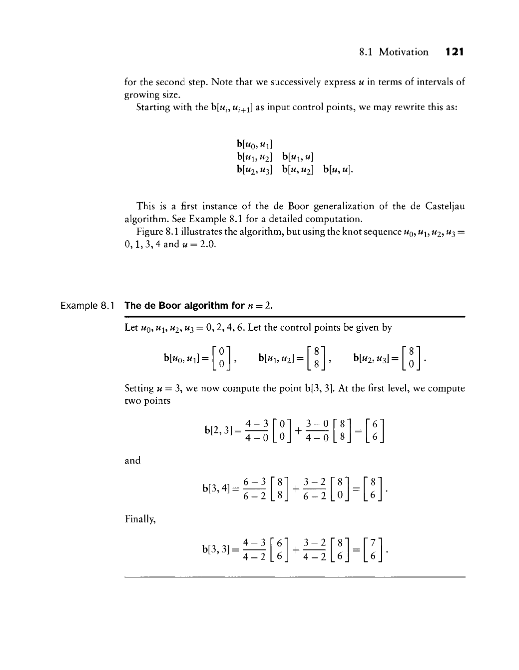
This is a first instance of the de Boor generalization of the de Casteljau
algorithm. See Example 8.1 for a detailed computation.
Figure 8.1 illustrates the algorithm, but using the knot sequence
WQ?
^l?
^2?
^3 =
0,1,
3,4 and ^ = 2.0.
Example 8.1 The de Boor algorithm for
n
= l.
Let
t/Q,
^1,
^2? ^3 = 0,2,4, 6. Let the control points be given by
h[uQ,
ui] =
b[wi,
U2]
=
b[w2,
u^]
=
0
Setting
w
= 3, we now compute the point b[3,
3].
At the first level, we compute
two points
and
Finally,
b[2,3]
=
b[3,4] =
4-3
4-0
6-3
6-2
+
3-0
4-0
[t\
[8]
_8_
3-2
+ 631
[8]
_0_
—
[8]
_6_
b[3,3]:
4-3
4-2
+
3-2
4-2
7
6