Farin G. Curves and Surfaces for CAGD. A Practical Guide

Подождите немного. Документ загружается.

92 Chapter 6 Bezier Curve Topics

Subdivision:

Derivative:

Integral:

B^(CO = ^B^WB;(0. (6.22)

±B^(t) = n[B^:l(t)-B^-\t)l

/ B^(x)dx=: V B"+i(0, (6.23)

Jo n +

^^^ ^

(x)dx

••

n-\-l

Three degree elevation formulas:

n + 1

Product:

(6.24)

tBIit) = l±lBl+lit), (6.25)

n +

Blit) = !l±l^B';+\t) + i±lBl+l(t). (6.26)

n +

B-(«)B;(«) = )^B-)"(«). (6.27)

6.11 Implementation

A C routine for degree elevation follows. Note that we have to treat the cases

/ = 0 and / = « + 1 separately; the program would not like the correspond-

ing nonexisting array elements. The program actually handles the rational

case,

which will be covered later. For the polynomial case, fill

with I's and

ignore wc.

6.12 Problems 93

void degree_elevdte(bx,by,wb,degree,ex,cy,wc)

/* input: two-d Bezier polygon in bx, by and with weights

in wb. Degree is degree.

Output:degree elevated curve in cx,cy and with weights in wc.

Note: for nonrational (polynomial) case, fill wc with I's.

6.12 Problems

*1 Prove (6.17).

* 2 Prove the relationship betv^een the "Bezier" and the Bernstein form for a

Bezier curve (6.14).

3 Prove that

* 4 With the result from the previous problem, prove

f;^(0 = n ( Bpi(x)dx.

PI The recursion formula for Bernstein polynomials is equivalent to the

de Casteljau algorithm. Devise a recursive curve evaluation algorithm for

curves in Chebychev form based on the recursion for Chebychev polyno-

mials.

Program it up and experiment!

P2 Program up degree reduction with some of the methods outlined in Section

6.4. Work with the Bezier polygon supplied in the file degred.dat.

This Page Intentionally Left Blank

Polynomial Curve

Constructions

1 olynomial interpolation is a fundamental concept for all of CAGD. Although

its uses are limited to low degrees, the basic concept still needs to be understood

in order to develop new algorithms. If the amount of data is too large for

interpolation to be successful, one uses approximation methods instead.

7.1 Aitken's Aigoritiim

A common problem in curve design is point data interpolation: from data points

with corresponding parameter values f^, find a curve that passes through the

p^.^

One of the oldest techniques to solve this problem is to find an interpo-

lating polynomial through the given points. That polynomial must satisfy the

interpolatory constraints

ip{ti)

= p-

/•

= 0,..., ^.

Several algorithms exist for this problem—any textbook on numerical analysis

will discuss several of them. In this section, we shall present a recursive technique

that is due to A. Aitken.

We have already solved the linear case, n=\ in Section 3.1. The Aitken

recursion computes a point on the interpolating polynomial through a sequence

The shape of the curve depends heavily on the parameter values

t^.

Methods for their

determination will be discussed later in the context of spline interpolation; see Section

9.6.

96 Chapter 7 Polynomial Curve Constructions

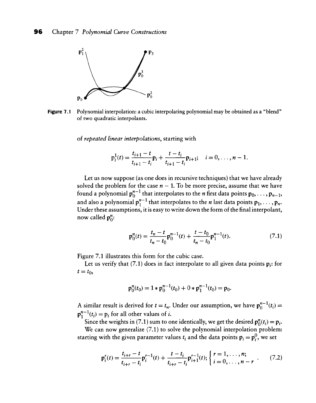
Figure 7.1 Polynomial interpolation: a cubic interpolating polynomial may be obtained as a "blend"

of two quadratic interpolants.

of repeated linear interpolations^ starting with

Let us now suppose (as one does in recursive techniques) that we have already

solved the problem for the case «

—

1. To be more precise, assume that we have

found a polynomial pQ~ that interpolates to the n first data points po,..., pn-h

and also a polynomial Pj~ that interpolates to the n last data points

pj,...,

p„.

Under these assumptions, it is easy to write down the form of the final interpolant,

now called p^:

PoW = T^Pr'W + —TPT'it)- (7.1)

Figure 7.1 illustrates this form for the cubic case.

Let us verify that (7.1) does in fact interpolate to all given data points

p^:

for

^ = ^05

Po(^o) =

* Po"^(^o) + 0 *

p'l-\to)

= Po.

A similar result is derived for t = tn. Under our assumption, we have pQ~ {fi) =

p\~^{ti)

for all other values of /.

Since the weights in (7.1) sum to one identically, we get the desired

p^{ti)

= p/.

We can now generalize (7.1) to solve the polynomial interpolation problem:

starting with the given parameter values tj and the data points p/ = p^ we set

7.1 Aitken's Algorithm 97

o • o o

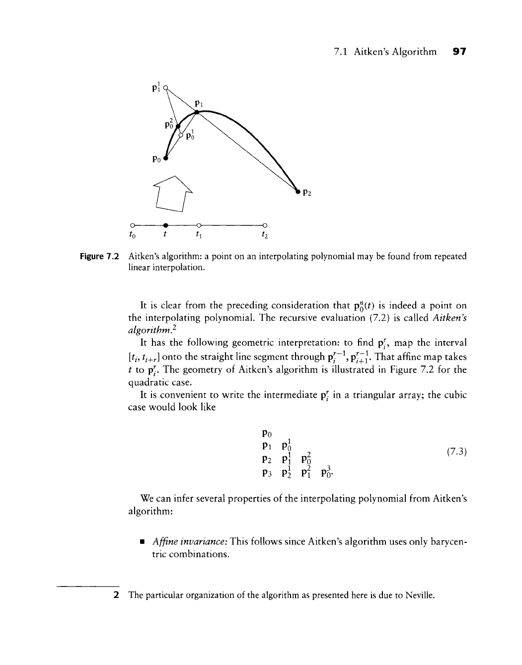
Figure 7.2 Aitken's algorithm: a point on an interpolating polynomial may be found from repeated

linear interpolation.

It is clear from the preceding consideration that p^(t) is indeed a point on

the interpolating polynomial. The recursive evaluation (7.2) is called Aitken's

algorithm?

It has the follow^ing geometric interpretation: to find p[, map the interval

[tj,

tj^j.]

onto the straight line segment through pp ,

p^~^.

That affine map takes

t to p^. The geometry of Aitken's algorithm is illustrated in Figure 7.2 for the

quadratic case.

It is convenient to write the intermediate p^ in a triangular array; the cubic

case would look like

^' 1 2 (7.3)

P2 Pi Po

P3 pi Pi Po-

We can infer several properties of the interpolating polynomial from Aitken's

algorithm:

Affine invariance: This follows since Aitken's algorithm uses only barycen-

tric combinations.

2 The particular organization of the algorithm as presented here is due to Neville.

98 Chapter 7 Polynomial Curve Constructions

Linear precision: If all p^ are uniformly distributed^ on a straight line

segment, all intermediate p[(^) are identical for r > 0. Thus the straight

line segment is reproduced.

No convex hull property: The parameter t in (7.2) does not have to lie

between ti and tij^y. Therefore, Aitken's algorithm does not use convex

combinations only:

PQ(^)

is not guaranteed to lie within the convex hull

of the p/. We should note, however, that no smooth curve interpolation

scheme exists that has the convex hull property.

No variation diminishing property: By the same reasoning, we do not

get the variation diminishing property. Again, no "decent" interpolation

scheme has this property. However, interpolating polynomials can augment

variation to an extent that renders them useless for practical problems.

7.2 Lagrange Polynomials

Aitken's algorithm allows us to compute a point p^(^) on the interpolating

polynomial through

+ 1 data points. It does not provide an answer to the

following questions: (1) Is the interpolating polynomial unique? (2) What is

a closed form for it? Both questions are resolved by the use of the Lagrange

polynomials L".

The explicit form of the interpolating polynomial p is given by

p(0 = ^P.Lf(0, (7.4)

where the L^ are Lagrange polynomials

Before we proceed further, we should note that the L" must sum to one in order

for (7.4) to be a barycentric combination and thus be geometrically meaningful;

we will return to this topic later.

3 If the points are on a straight line, but distributed unevenly, we will still recapture the

graph of the straight line, but it will not be parametrized linearly.

7.3 The Vandermonde Approach 99

We verify (7.4) by observing that the Lagrange polynomials are cardinal: they

satisfy

L-(?;) = 5,„, (7.6)

vv^ith

being the Kronecker delta. In other words, the /th Lagrange polynomial

vanishes at all knots except at the /th one, w^here it assumes the value 1. Because

of this property of Lagrange polynomials, (7.4) is called the cardinal form of the

interpolating polynomial p. The polynomial p has many other representations,

of course (v^e can rewrite it in monomial form, for example), but (7.4) is the only

form in which the data points appear explicitly.

We have thus justified our use of the term the interpolating polynomial. In

fact, the polynomial interpolation problem always has a solution, and it always

has a unique solution. The reason is that, because of (7.6), the L^ form a basis

of all polynomials of degree n. Thus, (7.4) is the unique representation of the

polynomial p in this basis. This is why one sometimes refers to all polynomial

interpolation schemes as Lagrange interpolation.^

We can now be sure that Aitken's algorithm yields the same point as does (7.4).

Based on that knowlege, we can conclude a property of Lagrange polynomials

that was already mentioned right after

{7.5)^

namely, that they sum to 1:

This is a simple consequence of the affine invariance of polynomial interpolation,

as shown for Aitken's algorithm.

7.5 The Vandermonde Approach

Suppose we want the interpolating polynomial p^ in the monomial basis:

/=0

4 More precisely, we refer to all those schemes that interpolate to a given set of data points.

Other forms of polynomial interpolation exist and are discussed later.

100 Chapter 7 Polynomial Curve Constructions

The standard approach to finding the unknown coefficients from the known data

is simply to write down everything one knows about the problem:

P^'C^o) = Po = ^0 + ^1^0 +

• • •

+ a„^Q,

P'^ih) = Pi = ao + ai^i + ... + a^t^,

P"(^«) = P« = ao + ^itn + . . . + ^n^n'

matrix form:

can shorten this

"Po"

-P«-

•

. t""

-J

-a„_

(7.8)

p = Ta. (7.9)

We already know that a solution a to this linear system exists, but one can

show independently that the determinant det T is nonzero (for distinct parameter

values ti). This determinant is known as the Vandermonde of the interpolation

problem. The solution, that is, the vector a containing the coefficients a^, can be

found from

= T-V

(7.10)

This should be taken only as a shorthand notation for the solution—not as an

algorithm! Note that the linear system (7.9) really consists of three linear systems

with the same coefficient matrix, one system for each coordinate. It is known

from numerical analysis that in such cases the LJJ decomposition of T is a more

economical way to obtain the solution a. This will be even more important when

we discuss tensor product surface interpolation in Section 15.4.

The interpolation problem can also be solved if we use basis functions other

than the monomials. Let {ff }^^o ^^ ^^^'^ ^ basis. We then seek an interpolating

polynomial of the form

p«(o-^cyp;w.

(7.11)

7=0

7.4 Limits of Lagrange Interpolation 101

This reasoning again leads to a linear system (three linear systems to be more

precise) for the coefficients c., this time with the generalized Vandermonde F:

F =

F"oit„)

F1(t„)

••

F"„(h)

••

F"„'it„)j

(7.12)

Since the F^ form a basis for all polynomials of degree n, it follows that the

generalized Vandermonde det F is nonzero.

Thus,

for instance, we are able to find the Bezier curve that passes through a

given set of data points: the F^ would then be the Bernstein polynomials B^.

1A Limits of Lagrange Interpolation

We have seen that polynomial interpolation is simple, unique, and has a nice

geometric interpretation. One might therefore expect this interpolation scheme

to be used frequently; yet it is virtually unknown in a design environment. The

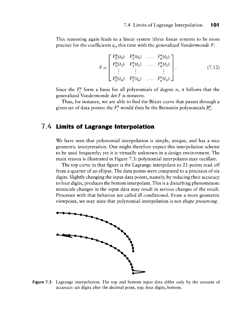
main reason is illustrated in Figure 7.3: polynomial interpolants may oscillate.

The top curve in that figure is the Lagrange interpolant to 21 points read off

from a quarter of an ellipse. The data points were computed to a precision of six

digits.

Slightly changing the input data points, namely, by reducing their accuracy

to four digits, produces the bottom interpolant. This is a disturbing phenomenon:

miniscule changes in the input data may result in serious changes of the result.

Processes with that behavior are called ill conditioned. From a more geometric

viewpoint, we may state that polynomial interpolation is not shape preserving.

Figure 7.3 Lagrange interpolation: The top and bottom input data differ only by the amount of

accuracy: six digits after the decimal point, top; four digits, bottom.