Farin G. Curves and Surfaces for CAGD. A Practical Guide
Подождите немного. Документ загружается.

102 Chapter 7 Polynomial Curve Constructions
This phenomenon is not due to numerical effects; it is actually inherent in
the polynomial interpolation process. Suppose we are given a finite arc of a
smooth curve c. We can then sample the curve at parameter values t^ and pass
the interpolating polynomial through those points. If we increase the number of
points on the curve, thus producing interpolants of higher and higher degree, we
would expect the corresponding interpolants to converge to the sampled curve
c. But this is not generally true: smooth curves exist for which this sequence of
interpolants diverges. This fact is dealt with in numerical analysis, where it is
known by the name of its discoverer: it is called the Runge phenomenon
[513].
Note, however, that the Runge phenomenon does not contradict the Weierstrass
approximation theorem!
As a second consideration, let us examine the cost of polynomial interpola-
tion, that is, the number of operations necessary to construct and then evaluate
the interpolant. Solving the Vandermonde system (7.8) requires roughly n^ op-
erations; subsequent computation of a point on the curve requires n operations.
The operation count for the construction of the interpolant is much smaller for
other schemes, as is the cost of evaluations (here piecewise schemes are far supe-
rior).
This latter cost is the more important one, of course: construction of the
interpolant happens once, but it may have to be evaluated thousands of times!
7.5 Cubic Hermite Interpolation
Polynomial interpolation is not restricted to interpolation to point data; we can
also interpolate to other information, such as derivative data. This leads to an
interpolation scheme that is more useful than Lagrange interpolation: it is called
Hermite interpolation. We treat the cubic case first, in which one is given a
set of points p/, associated parameter values ^/, and associated tangent vectors
(i.e.,
derivatives) m^. We just consider the case of two points po, pi and two
tangent vectors mo, m^, setting
tQ
= 0 and t^ = 1. The objective is to find a cubic
polynomial curve p that interpolates to these data:
P(0) = Po,
p(0) = mo,
p(l) = mi,
P(l)=Pi.
where the dot denotes differentiation.
We will write p in cubic Bezier form, and therefore must determine four Bezier
points bo,...,
b3.
Two of them are quickly determined:
7.5 Cubic Hermite Interpolation 103
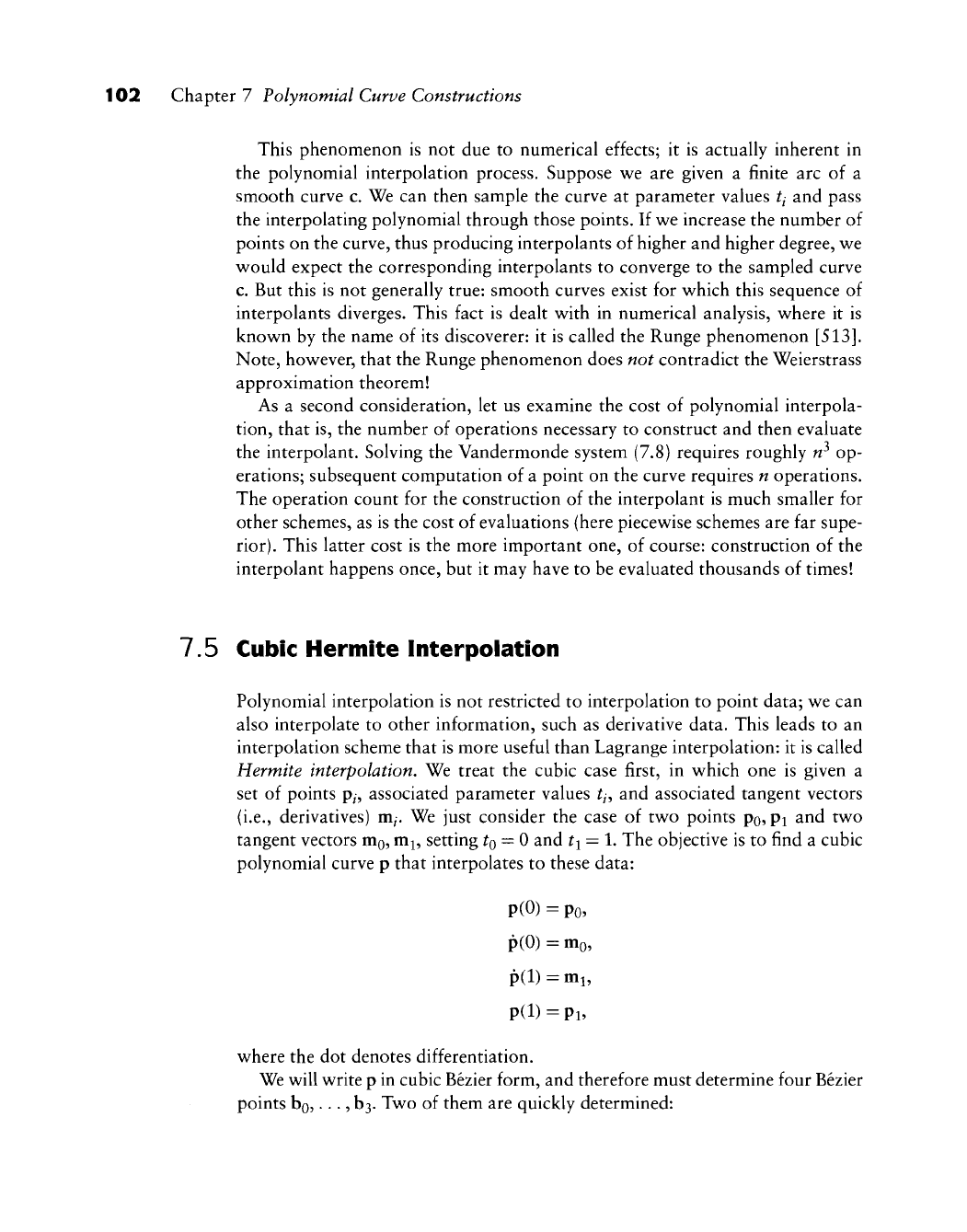
Figure 7.4 Cubic Hermite interpolation: the given data—points and tangent vectors—together v^ith
an interpolating cubic.
bo =
Po?
b3 = pi.
For the remaining two, we recall (from Section 5.3) the endpoint derivative for
Bezier curves:
p(0) = 3Abo, p(l) = 3Ab2.
We can easily solve for b^ and hi'-
u 1 1. 1
oi = Po + THIO, b2 = pi - -mi.
This situation—for the case of a general set of points and tangent vectors—is
shown in Figure 7.4.
Having solved the interpolation problem, we now attempt to write it in
cardinal form; we would like to have the given data appear explicitly in the
equation for the interpolant. So far, our interpolant is in Bezier form:
Pit) = poBlit) + Lo + ^mo j B\it) + Li - ^mi j Bl(t) + p^B^W-
To obtain the cardinal form, we simply rearrange:
Pit) = PoH^it) + moHlit) + m^Hlit) + PiH^it), (7.13)
104 Chapter 7 Polynomial Curve Constructions
\\H^\%i\\\\\\\\\\\\\]/^H^\\\
0 \J MX 3
III X. \Jr ill
R3 K PV
^1 MJ4 MM n\J
4
1
l^il
1
nin4^44-U44fTr Hj
M M
M
M M M ITM M M
^i
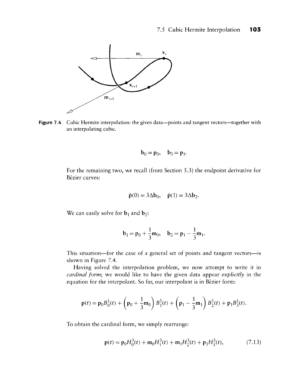
Figure 7.5 Cubic Hermite polynomials: the four Hf are shown over the interval
[0,1].
where we have set^
WQ(t) = Bl(t)+B\(t),
Hl(t) =
h\(t),
Hl(t) =
-lBl(t\
(7.14)
Hl(t)
=
Bl(t)-]-Bl{t).
The Hf are called cubic Hermite polynomials and are shown in Figure 7.5.
What are the properties necessary to make the Hf cardinal functions for the
cubic Hermite interpolation problem? They must be cardinal with respect to
evaluation and differentiation at t = 0 and
^
= 1, that is, each of the Hf equals 1
for one of these four operations and is 0 for the remaining three:
5 This is a deviation from standard notation. Standard notation groups by orders of
derivatives (i.e., first the two positions, then the two derivatives). The form of (7.13)
was chosen since it groups coefficients according to their geometry.
7.5 Cubic Hermite Interpolation 105
H3(0)
= 1, ^H3(0) = 0,
^H3(1)
= 0, H3(1) = 0,
d^ d^
H|(0)
= 0,
^H|(0)
= 0,
^^2^1)
= !,
H|(1)
= 0,
H|(0) = 0, AH|(0) = 0,
AH3(1)
= 0, H|(1) = 1.
Another important property of the Hf follows from the geometry of the
interpolation problem; (7.13) contains combinations of points and vectors. We
know that the point coefficients must sum to 1 if (7.13) is to be geometrically
meaningful:
This is, of course, also verified by inspection of (7.14).
Cubic Hermite interpolation has one annoying pecufiarity: it is not invariant
under affine domain transformations. Let a cubic Hermite interpolant be given
as in (7.13), that is, having the interval [0,1] as its domain. Now apply an affine
domain transformation to it by changing t to i = (1
—
t)a + tb, thereby changing
[0,1] to some
[a,
b].
The interpolant (7.13) becomes
Pit) = poH^(?) + moHld) + m^Hld) + PiH|(?), (7.15)
where the Hf(i) are defined through their cardinal properties:
H|(^)-0, jMl{a)^0,
j.Hlib)
= l, Hlib) = 0,
To satisfy these requirements, the new Hf must differ from the original Hf. We
obtain
106 Chapter 7 Polynomial Curve Constructions
j5ti\ _ u3/
Hl{t) = {b-a)Hl{t),
(7.16)
Hl{i) = {b-a)Hl(t\
where t e [0,1] is the local parameter of the interval
[a^
b\
Evaluation of (7.15) at
?
= ^ and i = b yields ^{d) = po, p(b) =
p^.
The deriva-
tives have changed, hov^ever. Invoking the chain rule, we find that dp(^)/d^ =
(b
— a)mQ
and, similarly, dp(fc)/d^ = (b
—
a)mi.
Thus an affine domain transformation changes the curve unless the defining
tangent vectors are changed accordingly—a drawback that is not encountered
with the Bernstein-Bezier form.
To maintain the same curve after a domain transformation, we must change
the length of the tangent vectors: if the length of the domain interval is changed by
a factor a, we must replace mg and
m^
by mo/a and m^/a, respectively. There is an
intuitive argument for this: interpreting the parameter as time, we assume we had
one time unit to traverse the curve. After changing the interval length by a factor
of 10, for example, we have 10 time units to traverse the same curve, resulting in
a much smaller speed of traversal. Since the magnitude of the derivative equals
that speed, it must also shrink by a factor of 10.
We also note that the Hermite form is not symmetric: if we replace ^ by 1
—
^
(assuming again the interval [0,1] as the domain), the curve coefficients cannot
simply be renumbered (as in the case of Bezier curves). Rather, the tangent vectors
must be reversed. This follows from the above by applying the affine map to the
[0,1] that maps that interval to
[1,
0], thus reversing its direction.
The dependence of the cubic Hermite form on the domain interval is rather
unpleasant—it is often overlooked and can be blamed for countless programming
errors by both students and professionals. We will use the Bezier form whenever
possible.
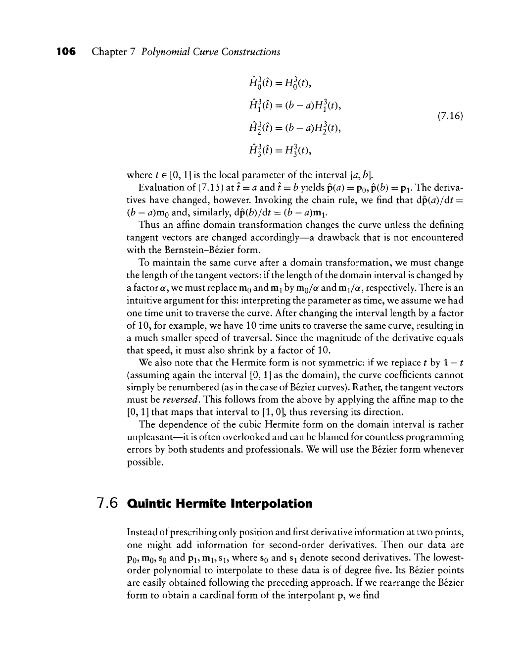
7.6 Quintic Hermite Interpolation
Instead of prescribing only position and first derivative information at two points,
one might add information for second-order derivatives. Then our data are
Po,
mo,
SQ
and
p^,
m^, s^, where So and s^ denote second derivatives. The lowest-
order polynomial to interpolate to these data is of degree five. Its Bezier points
are easily obtained following the preceding approach. If we rearrange the Bezier
form to obtain a cardinal form of the interpolant p, we find
1.1 Point-Normal Interpolation 107
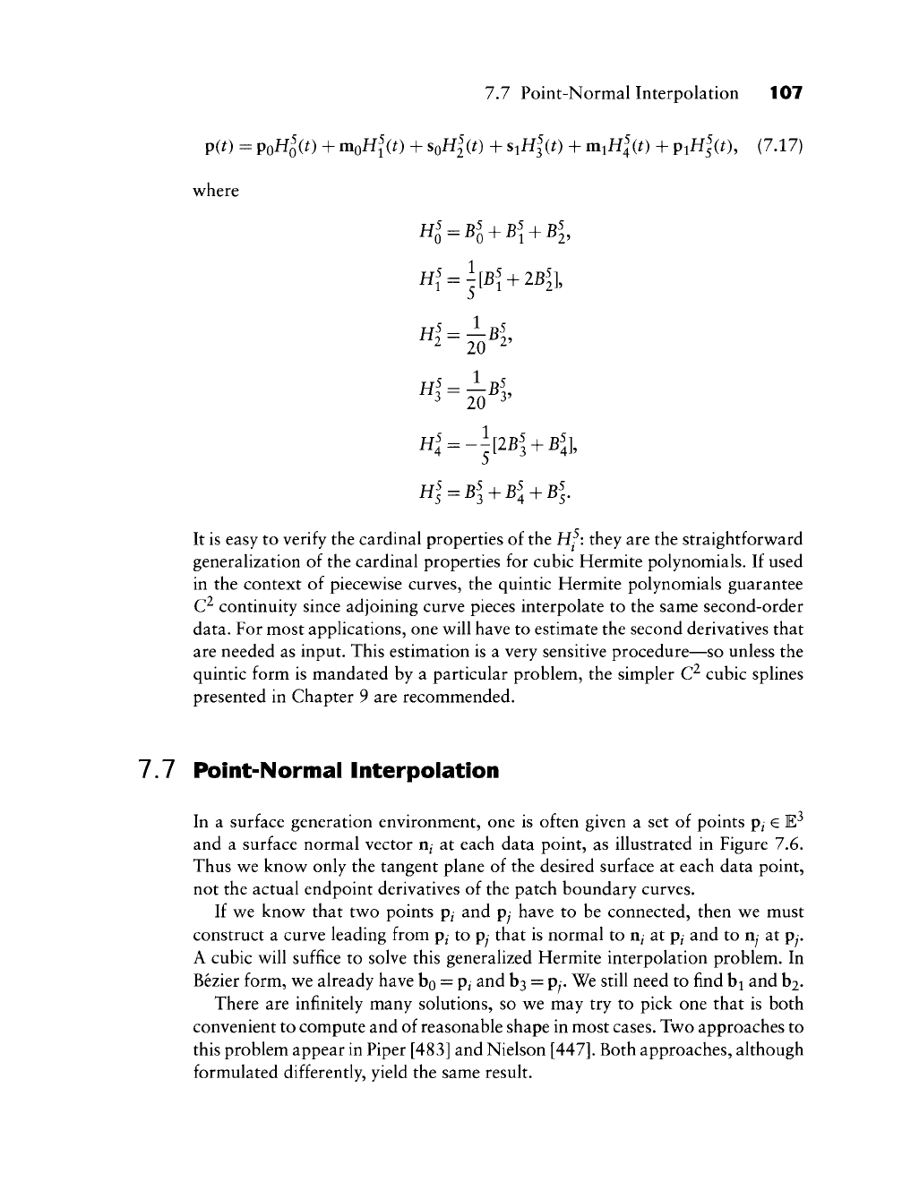
p(0 = PoH^W + moH^^W + soH|(0 + ^x^\if) + v^x^\(t) + PiH|(0, (7.17)
where
^ 20 ^
^5 1 R5
3 20 3
It is easy to verify the cardinal properties of the
H^^:
they are the straightforward
generalization of the cardinal properties for cubic Hermite polynomials. If used
in the context of piecewise curves, the quintic Hermite polynomials guarantee
C^ continuity since adjoining curve pieces interpolate to the same second-order
data. For most applications, one will have to estimate the second derivatives that
are needed as input. This estimation is a very sensitive procedure—so unless the
quintic form is mandated by a particular problem, the simpler C^ cubic splines
presented in Chapter 9 are recommended.
7.7 Point-Normal Interpolation
In a surface generation environment, one is often given a set of points p^
G
E^
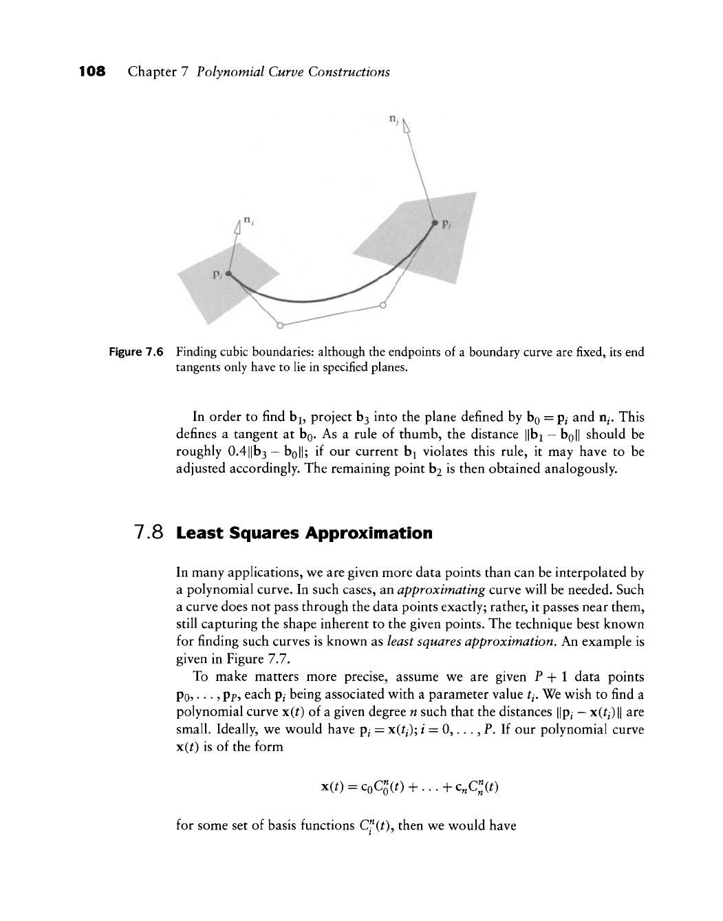
and a surface normal vector n^ at each data point, as illustrated in Figure 7.6.
Thus we know only the tangent plane of the desired surface at each data point,
not the actual endpoint derivatives of the patch boundary curves.
If we know that two points p/ and py have to be connected, then we must
construct a curve leading from p^ to py that is normal to n^ at p^ and to n. at p..
A cubic will suffice to solve this generalized Hermite interpolation problem. In
Bezier form, we already have bo = p/ and b3 =
py.
We still need to find b^ and h^.
There are infinitely many solutions, so we may try to pick one that is both
convenient to compute and of reasonable shape in most cases. Two approaches to
this problem appear in Piper [483] and Nielson
[447].
Both approaches, although
formulated differently, yield the same result.
108 Chapter 7 Polynomial Curve Constructions
Figure 7.6 Finding cubic boundaries: although the endpoints of a boundary curve are fixed, its end
tangents only have to lie in specified planes.
In order to find b^, project b3 into the plane defined by bo = p/ and n^. This
defines a tangent at bg. As a rule of thumb, the distance ||bi
—
boll should be
roughly 0.4||b3
—
boll; if our current b^ violates this rule, it may have to be
adjusted accordingly. The remaining point hi is then obtained analogously.
7.8 Least Squares Approximation
In many applications, v^e are given more data points than can be interpolated by
a polynomial curve. In such cases, an approximating curve w^ill be needed. Such
a curve does not pass through the data points exactly; rather, it passes near them,
still capturing the shape inherent to the given points. The technique best known
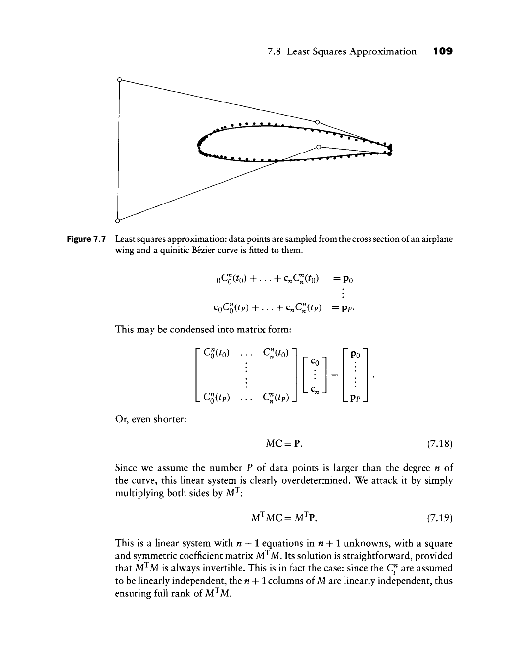
for finding such curves is knov^n as least squares approximation. An example is
given in Figure 7.7.
To make matters more precise, assume wt are given P + 1 data points
po,...,
pp, each pi being associated with a parameter value tj. We wish to find a
polynomial curve x(^) of a given degree n such that the distances ||p^
—
x(^/)
||
are
small. Ideally, we would have p^ =
x(^/);
/ = 0,..., P. If our polynomial curve
x(t) is of the form
xw = coqw + ... + c^c^w
for some set of basis functions
Cf(t),
then we would have
7.8 Least Squares Approximation 109
Figure 7.7 Least squares approximation: data points are sampled from the cross section of an airplane
wing and a quinitic Bezier curve is fitted to them.
oqc^o)
+ •.
•
+ c„qao) =Po
This may be condensed into matrix form:
Pp.
Clitp)
Or, even shorter:
qcfp)
J
MC = P.
Co
Po
LPPJ
(7.18)
Since we assume the number P of data points is larger than the degree n of
the curve, this hnear system is clearly overdetermined. We attack it by simply
multiplying both sides by M^:
M^MC = M^V. (7.19)
This is a linear system with
w
+ 1 equations in n-\-1 unknow^ns, with a square
and symmetric coefficient matrix M^M, Its solution is straightforward, provided
that M^M is always invertible. This is in fact the case: since the C" are assumed
to be linearly independent, the « +
1
columns of M are linearly independent, thus
ensuring full rank of M^M,
110 Chapter 7 Polynomial Curve Constructions
But is the solution meaningful? After all, we employed a rather crude trick in
going from (7.18) to (7.19). It turns out that our solution is not only meaningful—
in fact it is optimal.
In order to justify this claim (and also making it more precise), we give a
second derivation of (7.19).
Consider the following expression:
/"(Co,...,
c„) = ^ lip,- - x(^,)
(7.20)
/=0
If the curve x(t) does not deviate from the data points p/ by much, then f will
attain a small value. Ideally, if x were to pass through all pj exactly, we would
have
/"
= 0.
If we substitute the full definition of x(^) into (7.20), we obtain
/•(Co,...,
c^) = ^
/=0
j=0
(7.21)
We wish to find a set of
C/
such that the value of f becomes minimal. Since f is
a multivariate function of all components of the C/, that minimum is achieved if
f's
partials with respect to all these components vanish:
= 0; ^ = 0, ...,w; d = 1,2 or J = 1,2, 3,
where the superscript d labels the individual components of the c^^. Computing
the required derivatives yields
p
E
/=0
n
pf-J^cfCfit,)
'=0
Cl(t,) = 0; k =
0,,..,n;
J = 1,2 or J = 1,2, 3.
Upon rearranging, we see that this is identical to (7.19)!
7.9 Smoothing Equations
The solution to the least squares problem aims only at minimizing the error
function f in (7.20). It does not "care" about the shape of the resulting curve.
It may wiggle more than we would like, yet it is as close to the data points as
possible. Sometimes wiggles are undesired, even if closeness of approximation is
13 Smoothing Equations 111
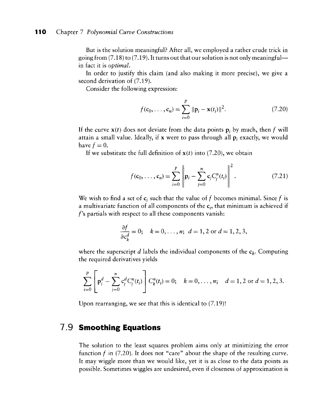
Figure 7.8 Least squares approximation: a degree 13 Bezier curve fitted to the airplane wing data
set.
lost. Typically, this is the case for noisy data: if the data points exhibit extraneous
wiggles, there is no point in trying to reproduce these. Figure 1.% shows a
"wiggly" control polygon. The next paragraph shows a way to improve the shape
of the approximating curve, albeit at the cost of deviating more from the given
data points.
We now assume that the basis functions
C^^{t)
are in fact the Bernstein polyno-
mials W^(t) and the unknown coefficients are contained in a vector B. Instead of
addressing the shape of the curve^ we will simply look at the shape of the control
polygon. Clearly, if the polygon behaves nicely, then so does the curve.
How do we measure the shape of a polygon.^ Many such measures are con-
ceivable; here, we pick one of the simplest ones. If all second differences A^hj are
small, then the polygon does not wiggle much. In addition to (7.18), we might
thus aim at also achieving all the following:
bo
—
2bi + b2
:0
b„_2 - 2b„
b.
=0.
This we abbreviate as
5B = 0.
(7.22)
If we simply append these equations to the overdetermined system (7.18), we
obtain one that is even more overdetermined:
M
S
B =
(7.23)
It is solved in the same way as (7.18), that is, by forming the symmetric linear
system of normal equations. The system is solvable because the coefficient matrix
of (7.23) still has n-\-l linearly independent columns, as inherited from the initial
matrix M.