Farin G. Curves and Surfaces for CAGD. A Practical Guide

Подождите немного. Документ загружается.

82 Chapter 6 Bezier Curve Topics

rb3 b

^^ hi

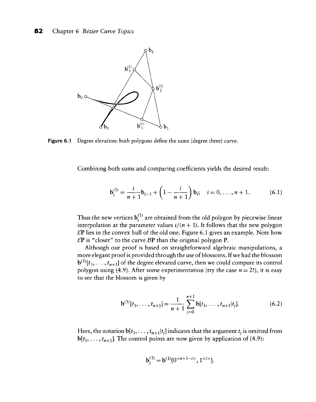
Figure 6.1 Degree elevation: both polygons define the same (degree three) curve.

Combining both sums and comparing coefficients yields the desired result:

+ 1 V

+ 1/

(6.1)

Thus the new vertices h- are obtained from the old polygon by piecewise linear

interpolation at the parameter values i/{n + 1). It follov^s that the nev^ polygon

£V lies in the convex hull of the old one. Figure 6.1 gives an example. Note how

SV is "closer" to the curve BV than the original polygon P.

Although our proof is based on straightforward algebraic manipulations, a

more elegant proof

provided through the use of

blossoms.

If we had the blossom

b(l)[

^1,...,

^„+i] of the degree elevated curve, then we could compute its control

polygon using (4.9). After some experimentation (try the case n = 2!), it is easy

to see that the blossom is given by

h^\h,..., ^„+i] = —- Y b[^i,...,

t^^^\t^\

(6.2)

Here, the notation b[^i,...,

t^^i\tj\

indicates that the argument tj is omitted from

b[^i,...,

^«+i]-

The control points are now given by application of (4.9):

b|^^

b^^^[o<"+^-^'^,r^"^].

6.2 Repeated Degree Elevation

Inspection of all terms that now arise in (6.2) reveals that the point b^_i appears

/ times and that the point b/ appears n-j-1

—

i times, thus reproving our previous

result.^

Degree elevation has important applications in surface design: for several

algorithms that produce surfaces from curve input,

is necessary that these

curves be of the same degree. Using degree elevation, v^e may achieve this by

raising the degree of all input curves to the one of the highest degree. Another

application lies in the area of data transfer between different CAD/CAM or

graphics systems: suppose you have generated a parabola (i.e., a degree two Bezier

curve),

and you want to feed it into a system that knows only about cubics. All

you have to do is degree elevate your parabola.

6.2 Repeated Degree Elevation

The process of degree elevation assigns a polygon £V to an original polygon P.

We may repeat this process and obtain a sequence of polygons P, f

^P,

and

so on. After r degree elevations, the polygon E^V has the vertices b^j ,.. .,

b|^^^^,

and each b

•

is explicitly given by

This formula is easily proved by induction.

Let us now investigate what happens

we repeat the process

degree

elevation again and again. As we shall see, the polygons E^V converge to the

curve that all of them define:

lim E'V = BV.

(6.4)

To prove this result,

fix

some parameter value

For each r, find the index

such that i/{n + r) is closest to

We can think of i/{n + r) as

parameter on

the polygon f

^P,

and as

-> oo, this ratio tends to t. We can now show (using

Stirling's formula) that

lim :±j;-^t\\-tr-i, (6.5)

1 Again, work out the example n = 2to build your confidence in this technique!

84 Chapter 6 Bezier Curve Topics

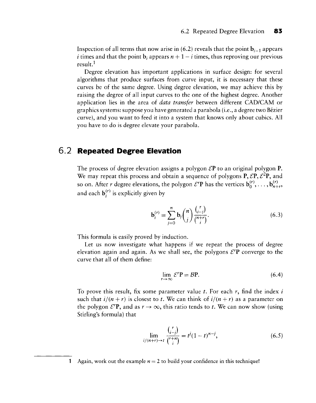
Figure 6.2 Degree elevation: a sequence of polygons approaching the curve that is defined by each

of them.

and therefore

i/{n+r)^t ^ c '

Equation {6.S) will look familiar to readers with a background in probability: it

states that the hypergeometric distribution converges to the binomial distribu-

tion.

Figure 6.2 shows an example of the limit behavior of the polygons £^V,

The polygons £^V approach the curve very slowly; thus our convergence result

has no practical consequences. However, it helps in the investigation of some

theoretical properties, as is seen in the next section.

The convergence of the polygons

£^V

to the curve was conjectured by

R. For-

rest [244] and proved in Farin

[187].

The preceding proof follows an approach

taken by

Zhou

[630].

Degree elevation may be generalized to "corner-cutting";

for a brief description, see Section 8.4.

6.5 The Variation Diminisiiing Property

We can now show that Bezier curves enjoy the variation diminishing property?

the curve BV has no more intersections with any plane than does the polygon P.

Degree elevation is an instance of piecewise linear interpolation, and we know

that operation is variation diminishing (see Section 3.2). Thus each £^V has fewer

intersections with a given plane than has its predecessor

£^^~^^V.

Since the curve is

The variation diminishing property was first investigated by I. Schoenberg [543] in the

context of B-spline approximation.

6.4 Degree Reduction 85

the limit of these polygons, we have proved our statement. For high-degree Bezier

curves, variation diminution may become so strong that the control polygon no

longer resembles the curve.

A special case is obtained for convex polygons: a planar polygon (or curve) is

said to be convex if it has no more than tw^o intersections with any plane. The

variation diminishing property thus asserts that a convex polygon generates a

convex curve. Note that the inverse statement is not true: convex curves exist

that have a nonconvex control polygon!

Though the variation diminishing property seems straightforward enough, it

is still not totally intuitive. Consider the following statement: two Bezier curves

with common endpoints do not intersect more often than their control polygons.

This appears to be true just after jotting down a few examples. Yet it is false, as

shown by Prautzsch

[494].

6.4 Degree Reduction

Degree elevation can be viewed as a process that introduces redundancy: a curve

is described by more information than is actually necessary. The inverse process

might seem more interesting: can we reduce possible redundancy in a curve

representation? More specifically, can we write a given curve of degree n-\-1

as one of degree n} We shall call this process degree reduction.

In general, exact degree reduction is not possible. For example, a cubic with a

point of inflection cannot possibly be written as a quadratic. Degree reduction,

therefore, can be viewed only as a method to approximate a given curve by one

of lower degree. Our problem can now be stated as follows: given a Bezier curve

with control vertices b|

;

/ = 0,.. .,

-h 1, can we find a Bezier curve with control

vertices

b^;

/ = 0,. . .,

that approximates the first curve in a "reasonable" way?

The equations for degree elevation may be combined into one matrix equation:

• •

• *

bo'

b„.

r K(1) n

L "n+1

{6.6)

Abbreviated:

MB = B^i\

M being a matrix with n-\-l rows and n-\-l columns.

(6.7)

86 Chapter 6 Bezier Curve Topics

In degree reduction, we seek to approximate a degee n + 1 curve by one of

degree n. In terms of (6.7), this means that we would be given

B^^^

and wish to

find

Clearly this is not possible in terms of solving a linear system, since M is

not a square matrix.

A trick will help: simply multiply both sides of (6.7) by M^, thus getting

M^MB = AfB^^\ (6.8)

Now we have a linear system for the unknown B with a square coefficient matrix

M^M—and any linear system solver will do the job!^

The linear system (6.8) is called the system of normal equations. It guarantees

that B is optimal in a least squares sense; for more discussion on this technique,

see Section 7.8. It is also optimal in the sense that the original and the degree

reduced curves are as close as possible in the least squares sense; see

[406].

In many cases, it might be desired that bg =

and b„ = b^^. Our least

squares solution will not meet these conditions in most cases—the simplest

solution is to enforce them after having found B.

Degree reduction has received a fair amount of attention in the literature; we

cite [97],

[182], [406], [472], [612].

6.5 Nonparametric Curves

We have so far considered three-dimensional parametric curves b(^). Now we

shall restrict ourselves to functional curves of the form y = f(x), where f denotes

a polynomial. These (planar) curves can be written in parametric form:

x(t)

yit)

fit)

Ht) =

We are interested in functions f that are expressed in terms of the Bernstein basis:

Note that now the coefficients bj are real numbers, not points. The bj therefore

do not form a polygon, yet functional curves are a subset of parametric curves

and therefore must possess a control polygon. To find it, we recall the linear

precision property of Bezier curves, as defined by (5.14). We can now write our

3 This linear system is

bidiagonal,

and may be solved much faster using simple backward

substitution.

6.6 Cross Plots 87

-0

/3-

/T\

1 /I

Z/J

1 1

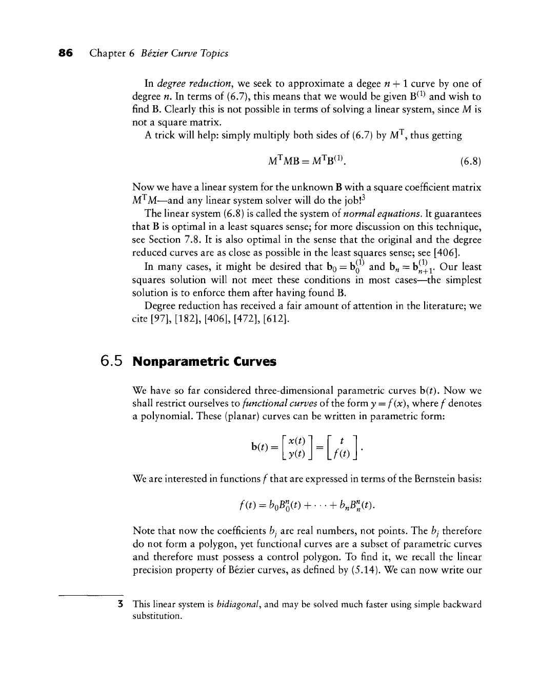
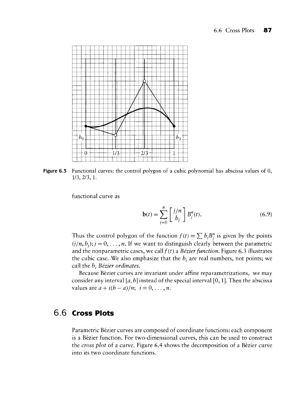
Figure 6.3 Functional curves: the control polygon of a cubic polynomial has abscissa values of 0,

1/3,2/3,1.

functional curve as

hit)

= J2

7=0

j/n

Blit).

(6.9)

Thus the control polygon of the function f(t) = ^ bjB^ is given by the points

(j/n,

bj);j

—

0,. . .,

If we want to distinguish clearly between the parametric

and the nonparametric cases, we call f(t) a Bezier function. Figure 6.3 illustrates

the cubic case. We also emphasize that the bi art real numbers, not points; we

call the bj Bezier ordinates.

Because Bezier curves are invariant under affine reparametrizations, we may

consider any interval

[a.,

instead of the special interval

[0,1].

Then the abscissa

values are a + i{b

—

a)/n; / = 0,..., ^.

6.6 Cross Plots

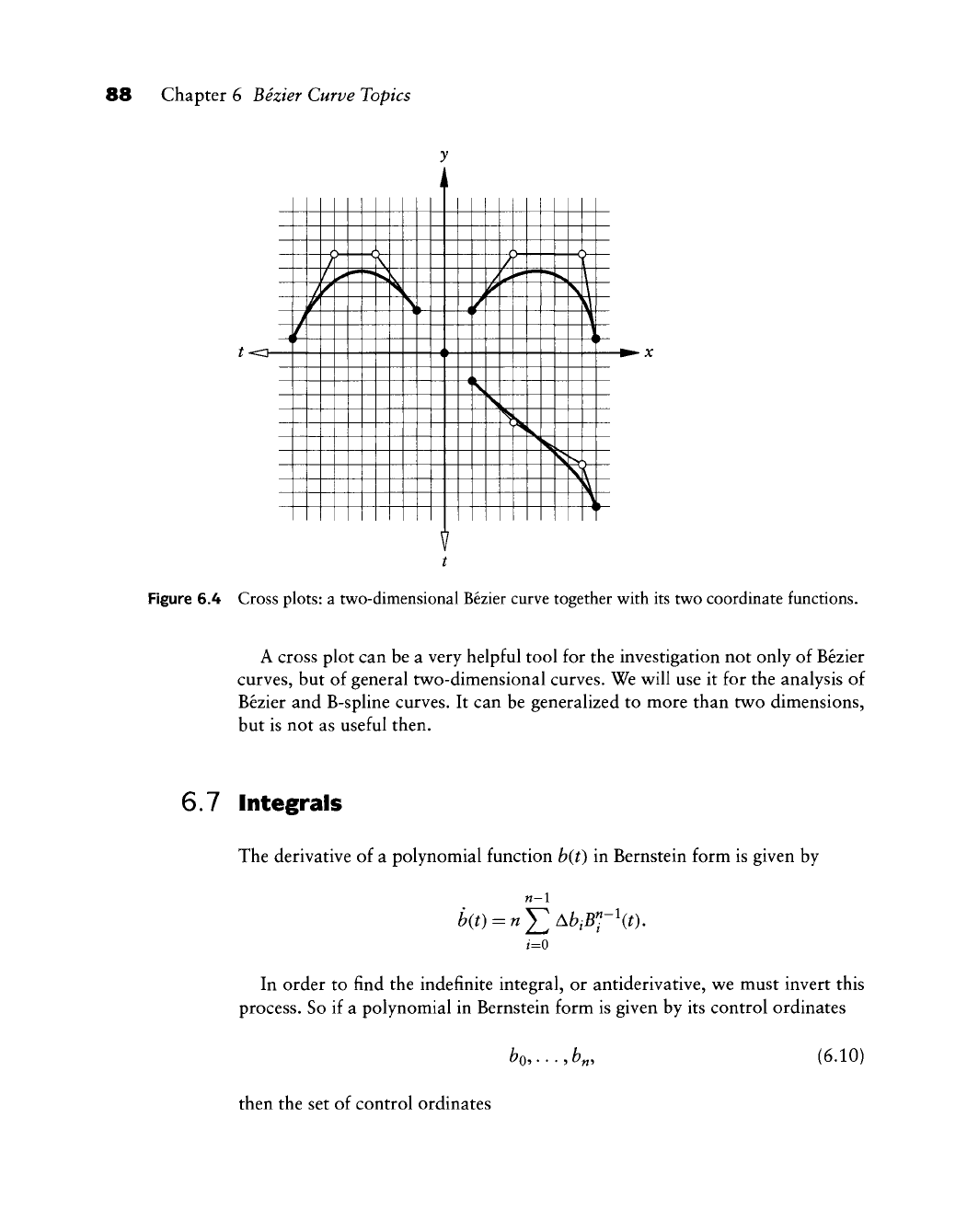
Parametric Bezier curves are composed of coordinate functions: each component

is a Bezier function. For two-dimensional curves, this can be used to construct

the cross plot of a curve. Figure 6.4 shows the decomposition of a Bezier curve

into its two coordinate functions.

88 Chapter 6 Bezier Curve Topics

?<H

Figure 6.4 Cross plots: a two-dimensional Bezier curve together with its two coordinate functions.

A cross plot can be a very helpful tool for the investigation not only of Bezier

curves, but of general tw^o-dimensional curves. We will use it for the analysis of

Bezier and B-spline curves. It can be generalized to more than tvvro dimensions,

but is not as useful then.

6.7 Integrals

The derivative of a polynomial function b{t) in Bernstein form is given by

n-l

i=0

In order to find the indefinite integral, or antiderivative, we must invert this

process. So if a polynomial in Bernstein form is given by its control ordinates

^05 • • •

^«9

(6.10)

then the set of control ordinates

6.8 The Bezier Form of a Bezier Curve 89

1 "

defines a polynomial B(t) whose derivative is exactly the one defined by the con-

trol ordinates (6.10). The scalar c is the usual constant encountered in indefinite

integration.

Since

[ b(t)dt = B(l)-B(0), (6.11)

we have immediately

/ bmt

-Tb,

(6.12)

^ +

The special case

gives

f Bnx)dx=-^; (6.13)

Jo ^ n + 1

that is, all basis functions B" (for a fixed n) have the same definite integral.

6.8 The Bezier Form of a Bezier Curve

In his work ([56], [57], [58], [59], [60], [61], [63], see also Vernet [599]), Bezier

did not use the Bernstein polynomials as basis functions. He wrote the curve b"

as a linear combination of functions Ff:

h"(t)^Y^c^F^(t),

(6.14)

,=0

where the F" are polynomials that obey the following recursion:

Ffit) ^{1- t)Ff-\t) + tFfzlit) (6.15)

with

foW = l, f;+iW = 0, FiW = l. (6.16)

90 Chapter 6 Bezier Curve Topics

Note that the third condition in the last equation is the only instance where the

definition of the F^ differs from that of the

B"!

An explicit expression for the F^

is given by

A consequence of (6.17) is that F^ = l for all n. Since F^it) >Oiorte

[0,1],

follows that (6.14) is not a barycentric combination of the

Cy.

In fact,

is a point

whereas the other

are vectors. The following relations hold:

co = bo, (6.18)

= Aby_i; ;>0. (6.19)

This undesirable distinction between points and vectors was abandoned soon

after Forrest's discovery that the Bezier form (6.14) of a Bezier curve could be

written in terms of Bernstein polynomials (see the appendix in [59]).

Comparing both forms, we notice that the Bernstein form is symmetric with

respect to t and 1

—

t, whereas the Bezier form is not. Let us assume the defining

coefficients b^ or C/ are affected by some numerical error and then let us check

the effect on the point x(l). In the Bernstein form, x(l) changes its value only if

b„ is in error. In the Bezier form, the value of x(l) is the sum of all errors in the

c^. If those cancel out, no harm is done—but if they do not, we may see serious

error accumulation!

6.9 The Weierstrass Approximation Tiieorem

One of the most important results in approximation theory is the Weierstrass

approximation theorem. S. Bernstein invented the polynomials that now bear

his name in order to formulate a constructive proof of this theorem (see Davis

[133]orKorovkin[364]).

We will give a "customized" version of the theorem, namely, we state it in the

context of parametric curves. So let c be a continuous curve that is defined over

[0,1].

For some fixed n, we can sample c at parameter values i/n. The points

c{i/n) can now be interpreted as the Bezier polygon of a polynomial curve x„:

X„W-^C(-)B^(0.

We say that x„ is the

n^"^

degree Bernstein-Bezier approximation to c.

6.10 Formulas

for

Bernstein Polynomials

are

next going

increase

the

density

of our

samples, that

is, we

increase

This generates

sequence

approximations x„, x^^^,....

The

Weierstrass

approximation theorem states that this sequence

polynomials converges

the curve

lim

x„(0 = c(0.

n-^OQ

At first sight, this looks like

handy

way to

approximate

given curve

polynomials:

just have

pick

degree

that

sufficiently large,

and we

are

to the

curve

as we

like. This

only theoretically true, however.

practice,

would have

choose values

of n in the

thousands

even millions

in order

obtain

reasonable closeness

of fit (see

Korovkin

[364] for

details).

The value

of the

theorem

therefore more

of a

theoretical nature.

shows

that every curve

may be

approximated arbitrarily closely

by a

polynomial curve.

6.10 Formulas

for

Bernstein Polynomials

This section

is a

collection

formulas; some appeared

in the

text, some

did not.

Credit

for

some

these goes

to R.

Farouki

and

V. Rajan

[225].

A Bernstein polynomial

defined

I 0

else.

The power basis

[f] and the

Bernstein basis {B^}

are

and

B"(t)

Y{-\i-'{ \{'\tL

(6.21)

Recursion:

B'i{t)

= (i-t)B';-\t)^tB';:i(t),