Fabien B. Analytical System Dynamics: Modeling and Simulation
Подождите немного. Документ загружается.


298 6 Dynamic System Analysis and Simulation
δW = v
1
δq
1
+ v
2
δq
2
+ v
bc
δq
c
− v
be
δq
e
.
Lagrange’s equations:
The kinetic coenergy for this model is T
∗
= 0 because there are no inductors.
The potential energy stored in the capacitors is
V =
q
2
2
2C
1
+
q
2
6
C
3
+
q
2
7
C
2
.
The dissipation function is
D =
1
2
R
0
f
2
2
+ R
1
f
2
4
+ R
2
f
2
3
+ R
C
f
2
5
+ R
E
f
2
8
+ R
3
f
2
6
.
Therefore, the Lagrangian DAEs (4.8) for this system are
˙q
1
− f
1
= 0, µ
1
− v
1
= 0, f
1
− f
4
− f
5
= 0,
˙q
2
− f
2
= 0,
q
2
C
1
+ R
0
f
2
+ µ
2
− v
2
= 0, f
2
− f
3
+ f
4
+ f
c
− f
e
= 0,
˙q
3
− f
3
= 0, R
2
f
3
− µ
2
= 0, f
5
− f
6
− f
c
= 0,
˙q
4
− f
4
= 0, R
1
f
4
− µ
1
+ µ
2
= 0, f
e
− f
7
− f
8
= 0,
˙q
5
− f
5
= 0, R
C
f
5
− µ
1
+ µ
3
= 0, f
e
− I
ES
I
F
+ I
s
I
R
= 0,
˙q
6
− f
6
= 0,
q
6
C
3
+ R
3
f
6
− µ
3
= 0, f
c
− I
s
I
F
+ I
CS
I
R
= 0,
˙q
7
− f
7
= 0,
q
7
C
2
− µ
4
= 0, I
R
− (e
αv
bc
− 1) = 0,
˙q
8
− f
8
= 0, R
E
f
8
− µ
4
= 0, I
F
− (e
αv
be
− 1) = 0.
˙q
e
− f
e
= 0, −µ
2
+ µ
4
+ v
be
= 0,
˙q
c
− f
c
= 0, µ
2
− µ
3
− v
bc
= 0,
In these equations µ
1
, µ
2
, µ
3
and µ
4
are the Lagrange multipliers associated
with the flow constraints (b). Also, the variables I
F
and I
R
are introduced
solely to simplify the presentation of the equations.
System simulation:
The DAEs given above are solved using the code ride with the following
model parameters; R
0
= 10
3
ohm, R
1
= 30 × 10
3
ohm, R
2
= 5.5 × 10
3
ohm, R
3
= 10 × 10
3
ohm, R
C
= 2 × 10
3
ohm, R
E
= 0.5 × 10
3
ohm,
C
1
= 10 ×10
−6
farad, C
2
= 100 ×10
−6
farad, C
3
= 10 ×10
−6
farad, v
1
= 12
volt, v
2
= 0.001 sin(2000πt) volt, (1/α) = 0.025 volt, I
ES
= 14.34 × 10
−15
amp, I
S
=
170
171
I
ES
amp, α
R
= 0.05, I
CS
= I
s
/α
R
amp.
The initial conditions used for this simulation are; µ
1
(0) = v
1
, f
4
(0) =
µ
1
(0)/R
1
, f
5
(0) = µ
1
(0)/R
C
, f
1
(0) = f
4
(0) + f
5
(0), f
2
(0) = −f
4
(0), f
6
(0) =
6.2 System Simulation 299
f
5
(0), q
2
(0) = −C
1
R
0
f
2
(0), and q
6
(0) = −C
3
R
3
f
6
(0). All other variables are
initialized to zero.
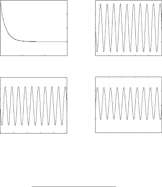
The solution to the DAEs in the interval 0 ≤ t ≤ 1.5 seconds is shown
Fig. 6.6. Here, the plot (i) shows v
R
3
(t), the voltage across the resistor R
3
.
As can be seen the system response approaches a steady-state after about 1
second. The plot (ii) shows v
R
3
(t) in the interval 1.49 ≤ t ≤ 1 second. This
plot clearly shows the input signal is amplified with gain of approximately
80. The plot (iii) shows the voltage at node C, i.e., v
C
= v
1
− R
C
f
5
, and
the plot (iv) shows the voltage at node B, i.e., v
B
= R
2
f
3
, in the interval
1.49 ≤ t ≤ 1.5. The results shown here are in good agreement with the
solution presented in Lamey (pp. 101).
0 0.5 1 1.5
−20
0
20
40
60
t
v
R3
(i)
1.49 1.492 1.494 1.496 1.498 1.5
−0.1
−0.05
0
0.05
0.1
t
v
R3
(ii)
1.49 1.492 1.494 1.496 1.498 1.5
7.3
7.35
7.4
7.45
7.5
v
C
t
(iii)
1.49 1.492 1.494 1.496 1.498 1.5
1.7955
1.796
1.7965
1.797
1.7975
v
B
t
(iv)
Fig. 6.6 Example 6.15
300 6 Dynamic System Analysis and Simulation
Example 6.16.
H
D
C
F
E
G
B
A
τ
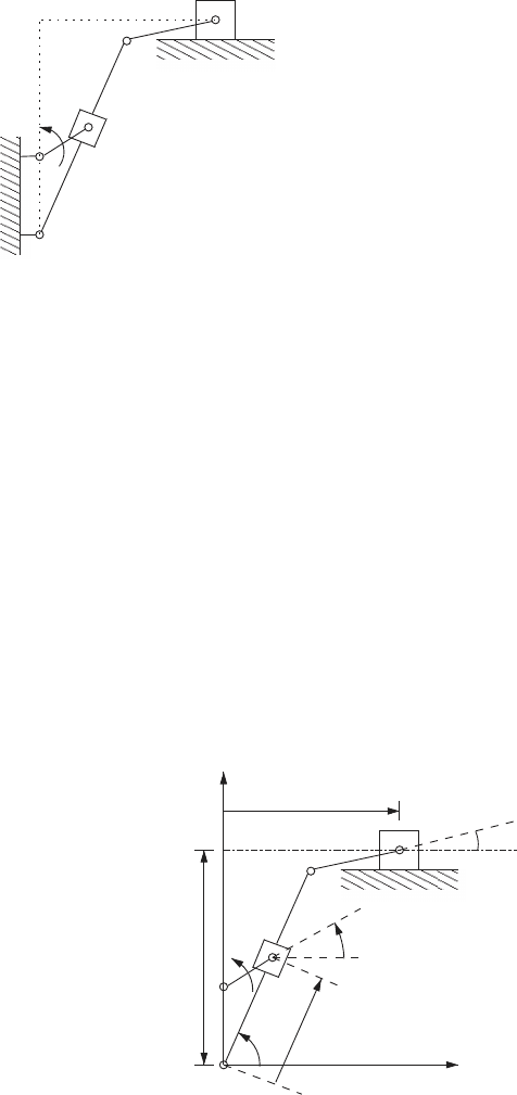
In the mechanism shown here an input
torque τ is applied to the crank BC. This
causes the slider at D to translate along
the link AE, while the link AE simulta-
neously rotates about A. Also, the motion
of the link EF causes the slider at G to
translate in the horizontal direction. The
motion of this device is such that the point
C has a circular path, while the point E
traverses a circular arc, and point F trans-
lates horizontally. In this device the links
BC, AE and EF are treated as uniform
bars. The sliders at D and G are treated
as lumped masses.
Kinematic analysis:
It is easy to verify that this mechanism has one degree of freedom. How-
ever, it will be convenient to use the following displacements to model the
system.
x
1
, y
1
: the location of the center of mass for link BC.
θ
1
: the angle link BC makes with the x-axis.
x
2
, y
2
: the location of the center of mass for link AE.
θ
2
: the angle link AE makes with the x-axis.
x
3
, y
3
: the location of the center of mass for link EF .
θ
3
: the angle link EF makes with the x-axis.
r
2
: the position of D along the link AE.
r
4
: the position of G along the x-axis.
The angles θ
1
, θ
2
, θ
3
, and the linear displacements r
2
and r
4
are shown in
the figure below.
4
θ
θ
θ
1
3
r
r
x
y
τ
l
AH
2
2

6.2 System Simulation 301
These 11 displacements are used to describe the 1 degree of freedom sys-
tem. Hence, we must establish 10 independent constraint equations to ac-
count for the ‘excess’ variables. We can obtain 6 of these equations by simply
stating the location of the mass centers for the links, i.e.,
φ
1
= x
1
−
l
BC
2
cos θ
1
= 0,
φ
2
= y
1
−
l
BC
2
sin θ
1
− l
AB
= 0,
φ
3
= x
2
−
l
AE
2
cos θ
2
= 0,
φ
4
= y
2
−
l
AE
2
sin θ
2
= 0,
φ
5
= x
3
− l
AE
cos θ
2
−
l
E F
2
cos θ
3
= 0,
φ
6
= y
3
− l
AE
sin θ
2
−
l
E F
2
sin θ
3
= 0.
Here, l
AB
is the length of link AB, l
BC
is the length of link BC, l
AE
is the
length of link AE, and l
EF
is the length of link EF .
The other 4 constraint equations are obtained by considering the closed-
loops
¯
AB +
¯
BC −
¯
AC = 0, and
¯
AE +
¯
EF −
¯
AH −
¯
HF = 0. These vector
equations give
φ
7
= l
BC
cos θ
1
− r
2
cos θ
2
= 0,
φ
8
= l
AB
+ l
BC
sin θ
1
− r
2
sin θ
2
= 0,
φ
9
= l
AE
cos θ
2
+ l
EF
cos θ
3
− r
4
= 0,
φ
10
= l
AE
sin θ
2
+ l
EF
sin θ
3
− l
AH
= 0,
where l
EF
is the length of link EF and l
AH
is the distance from A to H.
Applied effort analysis:
The virtual work done by the applied torque is
δW = τδθ
1
.
Lagrange’s equations:
The kinetic coenergy for this device is
T
∗
=
1
2
(m
BC
( ˙x
2
1
+ ˙y
2
1
) + I
BC
˙
θ
2
1
+ m
AE
( ˙x
2
2
+ ˙y
2
2
) + I
AE
˙
θ
2
2
+m
EF
( ˙x
2
3
+ ˙y
2
3
) + I
EF
˙
θ
2
3
+ m
D
l
2
BC
˙
θ
2
1
+ m
G
˙r
2
4
).
In this equation m
BC
denotes the mass of link BC, and I
BC
is the moment
of inertia of link BC about its center of mass. The other parameters in the
equation are similarly defined. Also, in this expression, the term
1
2
(m
BC
( ˙x
2
1
+
˙y
2
1
) + I
BC
˙
θ
2
1
) is the kinetic coenergy of the link BC, the term
1
2
(m
AE
( ˙x
2
2
+
˙y
2
2
) + I
AE
˙
θ
2
2
) is the kinetic coenergy of the link AE, the term
1
2
m
D
l
2
BC
˙
θ
2
1
is

302 6 Dynamic System Analysis and Simulation
the kinetic coenergy of the slider at D, and the term
1
2
m
G
˙r
2
4
is the kinetic
coenergy of the slider at G.
The potential energy and dissipation function are V = 0 and D = 0,
respectively.
Using these definitions the Lagrange’s equations of motion of the system
can be stated as
m
BC
¨x
1
+ λ
1
= 0,
m
BC
¨y
1
+ λ
2
= 0,
(I
BC
+ m
D
l
2
BC
)
¨
θ
1
+ l
BC
(λ
1
/2 − λ
7
) sin θ
1
+l
BC
(−λ
2
/2 + λ
8
) cos θ
1
= τ,
m
AE
¨x
2
+ λ
3
= 0,
m
AE
¨y
2
+ λ
4
= 0,
I
AE
¨
θ
2
+ l
AE
(λ
3
/2 + λ
5
− λ
9
+ r
2
λ
7
/l
AE
) sin θ
2
+l
AE
(−λ
4
/2 − λ
6
+ λ
10
− r
2
λ
8
/l
AE
) cos θ
2
= 0,
m
EF
¨x
3
+ λ
5
= 0,
m
EF
¨y
3
+ λ
6
= 0,
I
EF
¨
θ
3
+ l
EF
(λ
5
/2 − λ
9
) sin θ
3
+ l
EF
(−λ
6
/2 + λ
10
) cos θ
3
= 0,
−λ
7
cos θ
2
− λ
8
sin θ
2
= 0,
m
G
¨r
4
− λ
9
= 0,
(a)
where λ
1
, λ
2
, ···, λ
10
are the Lagrange multipliers associated with the dis-
placement constraints, φ
1
, φ
2
, ···, φ
10
.
System simulation:
The equations (a), along with the displacement constraints, define an index-3
differential-algebraic system. To obtain numerical solution to this problem we
will restate these equations in the GGL stabilized index-2 form. To do so let
us define the state displacement vector q = [x
1
, y
1
, θ
1
, x
2
, y
2
, θ
2
, x
3
, y
3
, θ
3
,
r
2
, r
4
]
T
, and let f = dq/dt be the corresponding flow vector. Then, (5.42)
gives

6.2 System Simulation 303
˙q
1
− f
1
+ ν
1
= 0,
˙q
2
− f
2
+ ν
2
= 0,
˙q
3
− f
3
+ l
BC
(ν
1
/2 − ν
7
) sin q
3
+ l
BC
(−ν
2
/2 + ν
8
) cos q
3
= 0,
˙q
4
− f
4
+ ν
3
= 0,
˙q
5
− f
5
+ ν
4
= 0,
˙q
6
− f
6
+ l
AE
(ν
3
/2 + ν
5
− ν
9
+ q
10
ν
7
/l
AE
) sin q
6
+ l
AE
(−ν
4
/2 − ν
6
+ ν
10
− q
10
ν
8
/l
AE
) cos q
6
= 0,
˙q
7
− f
7
+ ν
5
= 0,
˙q
8
− f
8
+ ν
6
= 0,
˙q
9
− f
9
+ l
EF
(ν
5
/2 − ν
9
) sin q
9
+ l
EF
(−ν
6
/2 + ν
10
) cos q
9
= 0,
˙q
10
− f
10
− ν
7
cos q
6
− ν
8
sin q
6
= 0,
˙q
11
− f
11
− ν
9
= 0,
m
BC
˙
f
1
+ λ
1
= 0,
m
BC
˙
f
2
+ λ
2
= 0,
(I
BC
+ m
D
l
2
BC
)
˙
f
3
+ l
BC
(λ
1
/2 − λ
7
) sin q
3
+l
BC
(−λ
2
/2 + λ
8
) cos q
3
= τ,
m
AE
˙
f
4
+ λ
3
= 0,
m
AE
˙
f
5
+ λ
4
= 0,
I
AE
˙
f
6
+ l
AE
(λ
3
/2 + λ
5
− λ
9
+ q
10
λ
7
/l
AE
) sin q
6
+l
AE
(−λ
4
/2 − λ
6
+ λ
10
− q
10
λ
8
/l
AE
) cos q
6
= 0,
m
EF
˙
f
7
+ λ
5
= 0,
m
EF
˙
f
8
+ λ
6
= 0,
I
EF
˙
f
9
+ l
EF
(λ
5
/2 − λ
9
) sin q
9
+ l
EF
(−λ
6
/2 + λ
10
) cos q
9
= 0,
−λ
7
cos q
6
− λ
8
sin q
6
= 0,
m
G
˙
f
11
− λ
9
= 0,
q
1
−
l
BC
2
cos q
3
= 0,
q
2
−
l
BC
2
sin q
3
− l
AB
= 0,
q
4
−
l
AE
2
cos q
6
= 0,
q
5
−
l
AE
2
sin q
6
= 0,

304 6 Dynamic System Analysis and Simulation
q
7
− l
AE
cos q
6
−
l
EF
2
cos q
9
= 0,
q
8
− l
AE
sin q
6
−
l
EF
2
sin q
9
= 0,
l
BC
cos q
3
− q
10
cos q
6
= 0,
l
AB
+ l
BC
sin q
3
− q
10
sin q
6
= 0,
l
AE
cos q
6
+ l
EF
cos q
9
− q
11
= 0,
l
AE
sin q
6
+ l
EF
sin q
9
− l
AH
= 0,
f
1
+
l
BC
2
f
3
sin q
3
= 0,
f
2
−
l
BC
2
f
3
cos q
3
= 0,
f
4
+
l
AE
2
f
6
sin q
6
= 0,
f
5
−
l
AE
2
f
6
cos q
6
= 0,
f
7
+ l
AE
f
6
sin q
6
+
l
EF
2
f
9
sin q
9
= 0,
f
8
− l
AE
f
6
cos q
6
−
l
EF
2
f
9
cos q
9
= 0,
−l
BC
f
3
sin q
3
− f
10
cos q
6
+ q
10
f
6
sin f
6
= 0,
l
BC
f
3
cos q
3
− f
10
sin q
6
− q
10
f
6
cos q
6
= 0,
−l
AE
f
6
sin q
6
− l
EF
f
9
sin q
9
− f
11
= 0,
l
AE
f
6
cos q
6
+ l
EF
f
9
cos q
9
= 0.
Here, ν
1
, ν
2
, ···, ν
10
are the multiplies associated with adjoining the flow
constraints
d
dt
φ
j
= 0, j = 1, 2, ···, 10, to the system.
These 42 differential-algebraic equations are solved to determine the be-
havior of the system. In this simulation we use the following model pa-
rameters; AH = 8 cm, AB = 4 cm, BC = 2 cm, AE = 8 cm, and
EF = 3 cm, m
BC
= 0.049 kg, I
BC
= 2.881 × 10
−6
kg-m
2
, m
AE
= 0.198
kg, I
AE
= 1.103 ×10
−4
kg-m
2
, m
EF
= 0.074 kg, I
EF
= 7.409 ×10
−6
kg-m
2
m
D
= 0.015 kg, and m
G
= 0.15 kg. The input torque is τ = 10(2 −
˙
θ
1
) N-m
The nonzero initial conditions are
θ
1
(0) = 0,
θ
2
(0) = tan
−1
(l
AB
/l
BC
),
θ
3
(0) = sin
−1
((l
AH
− l
AE
sin θ
2
(0))/l
EF
),
x
1
(0) = (l
BC
/2) cos θ
1
(0),
y
1
(0) = (l
BC
/2) sin θ
1
(0) + l
AB
,
x
2
(0) = (l
AE
/2) cos θ
2
(0),
y
2
(0) = (l
AE
/2) sin θ
2
(0),
x
3
(0) = l
AE
cos θ
2
(0) + (l
EF
/2)/ cos θ
3
(0),
y
3
(0) = l
AE
sin θ
2
(0) + (l
EF
/2)/ sin θ
3
(0),
r
2
(0) = (l
AB
+ l
BC
sin θ
1
(0))/ sin θ
2
(0),
r
4
(0) = l
AE
cos θ
2
(0) + l
EF
cos θ
3
(0),
6.2 System Simulation 305
¨
θ
1
(0) = 20/(I
BC
+ m
D
l
2
BC
).
In addition, we use ATOL=RTOL= 1.0 ×10
−4
, and INITIAL STEP SIZE= 1.0 ×
10
−4
.
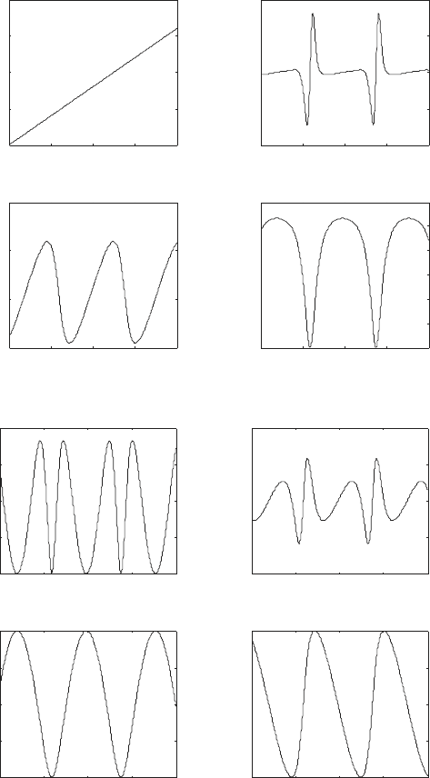
The results of this simulation are shown in Fig. 6.7 and Fig. 6.8. The plots
(i) and (ii) in Fig. 6.7 show the crank angle θ
1
and the angular velocity
˙
θ
1
.
Note that the torque input τ = 10(2−
˙
θ
1
) keeps θ
1
close to 2 radians/second.
The plots (iii) through (x) show the displacements and flows θ
2
,
˙
θ
2
, θ
3
,
˙
θ
3
, r
2
, ˙r
2
, r
4
, ˙r
4
, respectively. Notice that the device takes about 2 seconds
for the slider at G to travel from r
4
= 0.068 m to r
4
= −0.012 m. However,
it only takes about 1 second for the slider to travel from r
4
= −0.012 m to
r
4
= 0.068 m. For this reason this device is sometimes called a ‘quick return’
mechanism.
Finally, the plots (xi) and (xii) show the values of the constraints φ
7
, φ
8
,
φ
9
, and φ
10
. As can be seen these constraints are small relative to the desired
convergence tolerance (10
−4
.
Example 6.17.
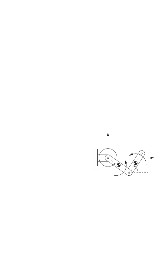
This example simulates the response of a pla-
nar R-R robot that is controlled to track a
desired trajectory. A schematic of the robot
is shown on the right. The angles q
1
and q
2
are the generalized displacements for the sys-
tem. The input torque to the link AB is τ
1
,
and the input torque to link BC is τ
2
. The
dynamic equations of motion for this system
are derived in Example 3.14. These equations
can be written as
2
B
A
x
y
C
q
q
τ
2
τ
1
1
M
11
M
12
M
21
M
22
¨q
1
¨q
2
+
f
1
f
2
=
τ
1
τ
2
, (a)
where
M
11
= I
1
+m
1
l
2
1
4
+m
2
l
2
1
, M
12
= M
21
=
m
2
l
1
l
2
2
cos(q
1
−q
2
), M
22
= I
2
+m
2
l
2
2
4
,
f
1
=
m
2
l
1
l
2
2
˙q
2
2
sin(q
1
− q
2
), f
2
= −
m
2
l
1
l
2
2
˙q
2
1
sin(q
1
− q
2
),
and the model parameters; m
1
, m
2
, I
1
, I
2
, l
1
and l
2
are defined in Example
3.14.
Our goal here is to have the robot angles follow a desired path specified
by angles q
1d
(t), and q
2d
(t). That is, we would like q
1
(t) = q
1d
(t) and q
2
(t) =
q
2d
(t). One way to accomplish this is to specify the input torques such that
306 6 Dynamic System Analysis and Simulation
0 2 4 6 8
0
5
10
15
20
(i)
t
θ
1
0 2 4 6 8
1.999
1.9995
2
2.0005
2.001
(ii)
t
dθ
1
/dt
0 2 4 6 8
1
1.5
2
2.5
(iii)
t
θ
2
0 2 4 6 8
−2
−1.5
−1
−0.5
0
0.5
1
(iv)
t
dθ
2
/dt
0 2 4 6 8
0
0.1
0.2
0.3
0.4
(v)
t
θ
3
0 2 4 6 8
−2
−1
0
1
2
(vi)
t
dθ
3
/dt
0 2 4 6 8
0.02
0.03
0.04
0.05
0.06
(vii)
t
r
2
0 2 4 6 8
−0.04
−0.02
0
0.02
0.04
(viii)
t
dr
2
/dt
Fig. 6.7 Example 6.16
6.2 System Simulation 307
0 2 4 6 8
−0.05
0
0.05
0.1
0.15
(ix)
t
r
4
0 2 4 6 8
−0.1
0
0.1
0.2
0.3
(x)
t
dr
4
/dt
0 2 4 6 8
−4
−3
−2
−1
0
1
2
x 10
−9
t
error
(xi)
φ
7
φ
8
0 2 4 6 8
−1
−0.5
0
0.5
1
x 10
−8
t
error
(xii)
φ
9
φ
10
Fig. 6.8 Example 6.16, continued.
τ
1
τ
2
=
M
11
M
12
M
21
M
22
¨q
1d
¨q
2d
+
f
1
f
2
− 2ζω
˙q
1
− ˙q
1d
˙q
2
− ˙q
2d
− ω
2
q
1
− q
1d
q
2
− q
2d
, (b)
where ζ > 0 and ω > 0 are constants. Then, using (b) in (a) gives
¨e + 2ζω ˙e + ω
2
e = 0, (c)
where e = [(q
1
− q
1d
), (q
2
− q
2d
)]
T
is the tracking error. We see that this
error satisfies a linear second-order differential equation, (c), with constant
coefficients. Moreover, the coefficients of this error differential equation can
be selected arbitrarily. If we set ζ > 1 then the solution to (c) is called
‘overdamped’ and is of the form
e
i
(t) = a
i1
e
λ
1
t
+ a
2i
e
λ
2
t
, i = 1, 2, (d)
where λ
1
= −ω(ζ +
p
ζ
2
− 1), λ
1
= −ω(ζ −
p
ζ
2
− 1). The coefficients a
1i
,
and a
2i
, i = 1, 2 depend on the initial conditions e(0), and ˙e(0). Since, λ
1
< 0
and λ
2
< 0 we see from (d) that
lim
t→∞
e(t) = 0.
