Everitt B.S. The Cambridge Dictionary of Statistics

Подождите немного. Документ загружается.

P is known as a transition matrix. The ijth element of P

gives the n-step transition

probability. If the limit as n !1is π

then the π

s constitute the stationary distribution of

the chain. [Statistics in Civil Engineering, 1997, A. V. Metcalfe, Edward Arnold, London.]

Markov chain Monte Carlo methods (MCMC): Powerful methods for indirectly simulating

random observations from complex, and often high dimensional probability distributions.

Originally used in image processing for the restoration of blurred or distorted pictures, the

technique has now become of considerable importance in many branches of statistics, in

particular in applications of

Bayesian inference

where the integrations needed to evaluate the

posterior distribution

itself or particular features of interest such as moments, quantiles, etc.,

have, until recently, been a source of considerable practical difﬁculties. But although most

applications of MCMC have been in Bayesian inference, the methods are often also

extremely useful in classical

likelihood

calculations. In general terms the problem attacked

by MCMC methodology is that of obtaining characteristics of interest (for example, mean,

variance, etc.) of the

marginal distribution

, f(x) arising from a given

joint distribution

gðx; y

; ...; y

Þ as

f ðxÞ¼



gðx; y

; ...; y

Þdy

...dy

The most natural and straightforward approach would be to calculate f(x) and then use it to

obtain the required characteristics. In general, however, the necessary integrations are

extremely difﬁcult to perform, either analytically or numerically. MCMC methods effec-

tively allow generation of samples from f(x) without requiring f(x) explicitly. By simulating a

large enough sample, the mean, variance or any other characteristic of f(x) (or f(x) itself) can

be calculated to any desired degree of accuracy. The essential feature of the MCMC

approach is a cleverly constructed

Markov chain

, the

stationary distribution

of which is

precisely the distribution of interest f. A number of different methods are available for

creating this Markov chain consisting of a sequence of random variables fX

; X

; ...g.

The Metropolis–Hastings algorithm, for example, samples at each stage a candidate point Y

from a so-called proposal distribution that may depend on the current point X

. The candidate

point is then accepted with probability αðX

; Y Þ where

αðX ; Y Þ¼minð1;

f ðY ÞqðX jY Þ

f ðX ÞqðY jX Þ

and q is the proposal distribution. If the candidate point is accepted, the next state becomes

tþ1

¼ Y otherwise X

tþ1

¼ X

and the chain does not move. Remarkably, the proposal

distribution q can take any form and the stationary dis tribution of the chain will still be f.

An example of the application of this algorithm in a simple case is shown in Fig. 92.The

most widely used form of MCMC in statistical applications is Gibbs sampling where, for

two variables for example, a sample from f(x) is generated by sam pling instead from the

two conditional distributions, hðxjyÞ and rðy jxÞ. So now, beginning with an initial value

a sequ ence fY

; X

; Y

; X

; Y

; X

; ...; Y

; X

g is generated by sampling X

from hð:jY

and Y

j+1

from rð:jX

Þ. Under reasonably general conditions the distribution of X

con-

verges to f(x)ask !1.Sofork large enough the ﬁnal observation in the sequence is

effectively a s ample point from f (x). See also data aug mentation algorithm.[Markov

Chain Monte Carlo in Practice, 1996, edited by W. R. Gilks, S. Richardson and D. J.

Spiegelhalter, C hapman and Hall/CRC Press, London.]

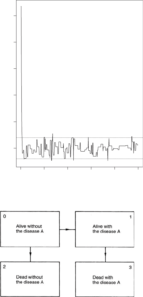
Markov illness^death model: A model in which live individuals are classiﬁed as either having,

or not having, a disease A, and then move between these possibilities and death as indicated

in Fig. 93.[Medical Decision Making, 1994, 14, 266–72.]

269

Markov inequality: See Chebyshev’s inequality.

M arkov process: Synonym for continuous time Maskov chain.

Marquisof Lansdowne(1780^1863): William Petty Fitzmaurice Lansdowne was a British Whig

politician who became the ﬁrst President of the Royal Statistical Society. He was a champion of

Catholic emancipation, the abolition of the slave-trad e and the cause of popular education.

Iteration

100 200 300 400 500

0 510152025

Fig. 92 Markov chain Monte Carlo methods illustrated by 500 iterations from the Metropolis

algorithm with stationary distribution N(0, 1) and proposed distribution N(x, 5.5).

Fig. 93 Markov illness–

death model diagram.

270

MARS: Acronym for multivariate adaptive regression splines.

Martingale: In a gambling context the term originally referred to a system for recouping losses by

doubling the stake after each loss. The modern mathematical concept can also be viewed in

such terms as a mathematical formalization of the concept of a ‘fair’ game deﬁned as one in

which the expected size of the gambler’s bank after the nth game given the results of all

previous games is unchanged from the size after the (n − 1)th game, i.e. the gambler’s

average gain or loss after each game, given the previous history of the games is zero. More

formally the term refers to a

stochastic process

, or a sequence of random variables S

; S

; ...,

which is such that the expected value of the ðn þ1Þth random variable conditional on the

values of the ﬁrst n, equals the value of the nth random variable, i.e.

E ð S

nþ1

; S

; ...; S

Þ¼S

n  1

so that E(S

) does not depend on n.[Discrete Parameter Martingales, 1975, J. Neveu, North

Holland, Amsterdam.]

Masking: A term usually applied in the context of a sample containing multiple

outliers

whose presence

prevents many methods from detecting them. May also be used as a synonym for

blinding

[Clinical Trials in Psychiatry, 2008, B. S. Everitt and S. Wessely, Wiley, Chichester.]

M atc hed case-contr o l study: See retrospective study.

Matched pairs: A term used for observations arising from either two individuals who are individ-

ually matched on a number of variables, for example, age, sex, etc., or where two observa-

tions are taken on the same individual on two separate occasions. Essentially synonymous

with paired samples.

Matched pairs t-test: A

Student’s t-test

for the equality of the means of two populations, when the

observations arise as

paired samples

. The test is based on the differences between the

observations of the matched pairs. The

test statistic

is given by

t ¼



ﬃﬃﬃ

where n is the sample size,



d is the mean of the differences, and s

their standard deviation. If

the null hypothesis of the equality of the population means is true then t has a

Student’s

-distribution with n − 1 degrees of freedom. [SMR Chapter 9.]

Matched set: See one:m matching.

Matching: The process of making a study group and a comparison group comparable with respect to

extraneous factors. Often used in

retrospective studies

when selecting cases and controls to

control variation in a response variable due to sources other than those immediately under

investigation. Several kinds of matching can be identiﬁed, the most common of which is

when each case is individually matched with a control subject on the matching variables,

such as age, sex, occupation, etc. When the variable on which the matching takes place is

continous it is usually transformed into a series of categories (e.g. age), but a second method

is to say that two values of the variable match if their difference lies between deﬁned limits.

This method is known as caliper matching. Also important is group matching in which the

distributions of the extraneous factors are made similar in the groups to be compared. See

also paired samples. [SMR Chapter 5.]

Matching coefficient: A

similarity coefﬁcient

for data consisting of a number of binary variables

that is often used in

cluster analysis

. Given by

271

a þb þ c þd

where a, b, c and d are the four frequencies in the two-by-two cross-classiﬁcation of the

variable values for subjects i and j. See also Jaccard coefﬁcient.[Cluster Analysis,

4th edition, 2001, B. S. Everitt, S. Landau and M. Leese, Arnold, London.]

Matching distribution: A probability distribution that arises in the following way. Suppose that a

set of n subjects, numbered 1; ...; n respectively, are arranged in random order, then it is the

distribution of the number of subjects for which the position in the random order equals the

number originally assigned to them. Found from application of

Boole’s formula

to be

PrðX ¼ xÞ¼½x!

1

f1 ð1!Þ

1

þð2!Þ

1

þþð1Þ

nx

ðn xÞ!

1

g x ¼ 0; 1; ...; n

Note that PrðX ¼ n  1Þ¼0. [Univariate Discrete Distributions, 2005, N. L. Johnson,

A. W. Kemp and S. Kotz, Wiley, New York.]

M aternal mortality: A maternal death is the death of a woman while pregnant, or within 42 days of

the termination of pregnancy, from any cause related to or aggravated by the pregnancy or its

management, but not from accidental or incidental causes. Some 585 000 women a year die

as a result of maternal mortality, 99% of them in the developing world. [World Health

Statistics Quarterly, 1996, 49,77–87.]

Mathematica: A fully integrated software environment for technical and scientiﬁccomputingthat

combines numerical and symbolic computation. See also Maple. [http://www.wolfram.com/ ]

Mathisen’s test:

A distribution free test

for the

Behrens–Fisher problem

.[Robust Non-parametric

Statistical Methods, 1998, T. P. Hettmansperger and J. W. McKean, Arnold, London.]

Mat rixex pone ntialtr a nsfo r ma ti on: A transformation for any p×pmatrix A,deﬁned as follows:

C ¼ expðAÞ¼

s¼0

where A

is the p×pidentity matrix and A

denotes ordinary matrix multiplication of A, s

times. Used in the modelling of a

variance–covariance matrix

in particular in studying the

dependence of the covariances on explanatory variables. [International Journal of Applied

Mathematics, 2001, 7, 289–308.]

Mauchlytest: A test that a

variance–covariance matrix

of pairwise differences of responses in a set of

longitudinal data is a scalar multiple of the identity matrix, a property known as sphericity.

Of most importance in the analysis of

longitudinal data

where this property must hold for the

F-tests in the

analysis of variance

of such data to be valid. See also compound symmetry,

Greenhouse–Geisser correction and Huynh–Feldt correction. [MV2 Chapter 13.]

MAVE method: Abbreviation for minimum average variance estimation method.

M aximum a posterior i esti mate (MA P): Essentially the mode of a

posterior distribution

Often used as a measure of location in image analysis applications. [Markov Chain Monte

Carlo in Practice, 1996, W. R. Gilks, S. Richardson, and D. J. Spiegelhalter, Chapman and

Hall/CRC Press, London.]

M axi mum entr op y pr i nc i p le: A principle which says that to assign probabilities using limited

information, the

entropy

of the distribution, S, should be maximized where

S ¼

logðp

subject to the constraints of known expectation values. [The Statistician , 1998, 4, 629–41.]

272

M axi mum F-rati o: Equivalent to

Hartley’s test

. See also Bartlett’s test and Box’s test.

Maximu m l ik e lihood est imati on: An estimation procedure involving maximization of the

like-

lihood

or the

log-likelihood

with respect to the parameters. Such estimators are particularly

important because of their many desirable statistical properties such as

consistency

,and

asymptotic efﬁciency

. As an example consider the number of successes, X,inaseriesof

random

variables

from a

Bernoulli distribution

with success probability p. The likelihood is given by

PðX ¼ xjpÞ¼



ð1 pÞ

nx

Differentiating the log-likelihood, L, with respect to p gives



n x

1 p

Setting this equal to zero gives the estimator

p ¼ x=n. See also EM algorithm. [KA2

Chapter 18.]

M aximum lik eli hood esti mator: The estimator of a parameter obtained from applying

maxi-

mum likelihood estimation

Maximumno rmedresidua l: A statistic that may be used to test for a single

outlier

, when ﬁtting a

linear model. Deﬁned as the maximum of the absolute values of the normed residuals, that is

jzj

ð1Þ

¼ maxfjz

j; jz

j; ...; jz

where z

¼ e

=ð

i¼1

and e

is the usual residual, namely the observed minus the

predicted value of the response variable. [Annals of Mathematical Statistics, 1971, 42,

35–45.]

Maxwell, Albert Ernest (1916^1996): Maxwell was educated at the Royal School, Cavan and

at Trinity College, Dublin where he developed interests in psychology and mathematics. His

ﬁrst career was as school teacher and then headmaster at St. Patrick’s Cathedral School,

Dublin. In 1952 Maxwell left school teaching to take up a post of lecturer in statistics at the

Institute of Psychiatry, a post graduate school of the University of London. He remained at

the Institute until his retirement in 1978. Maxwell’s most important contributions were in

multivariate analysis

, particularly

factor analysis

. He died in 1996 in Leeds, UK.

M ayo-Smith, R ichard ( 1 854^1 901): Born in Troy, Ohio, Mayo-Smith graduated from Amherst

college eventually obtaining a Ph.D. Joined the staff of Columbia College as an instructor in

history and political science. One of the ﬁrst to teach statistics at an American university, he

was also the ﬁrst statistics professor to open a statistical laboratory. Mayo-Smith was made

an Honorary Fellow of the Royal Statistical Society in 1890, the same year in which he was

elected a member of the National Academy of Sciences.

MAZ experiments:

Mixture–amount experiments

which include control tests for which the total

amount of the mixture is set to zero. Examples include drugs (some patients do not receive

any of the formulations being tested) fertilizers (none of the fertilizer mixtures are applied to

certain plots) and paints/coatings (some specimens are not painted/coated). [Experiments

with Mixtures; Design Models and The Analysis of Mixture Data, 1981, J. A. Cornell, Wiley,

New York.]

MCAR: Abbreviation for missing completely at random.

McCabe^Tremayne test: A test for the

stationarity

of particular types of

time series

.[Annals of

Statistics, 1995, 23, 1015–28.]

273

MCMC: Abbreviation for Markov chain Monte Carlo method.

MCML : Abbreviation for Monte Carlo maximum likelihood.

McNemar’s test: A test for comparing proportions in data involving

paired samples

. The test

statistic is given by

ðb cÞ

b þc

where b is the number of pairs for which the individual receiving treatment A has a positive

response and the individual receiving treatment B does not, and c is the number of pairs for

which the reverse is the case. If the probability of a positive response is the same in each group,

then X

has a

chi-squared distribution

with a single degree of freedom. [SMR Chapter 10.]

MCP : Abbreviation for minimum convex polygon.

MDL : Abbreviation for minimum description length.

MDP : Abbreviation for minimum distance probability.

MDS: Abbreviation for multidimensional scaling.

Mean: A measure of location or central value for a continuous variable. For a deﬁnition of the

population value see

expected value

. For a sample of observations x

; x

; ...; x

the measure

is calculated as



x ¼

i¼1

Most useful when the data have a

symmetric distribution

and do not contain

outliers

. See

also median and mode. [SMR Chapter 2.]

Mean and dispersion additive model (MADAM): A ﬂexible model for variance hetero-

geneity in a normal error model, in which both the mean and variance are modelled using

semi-parametric additive models. [Statistics and Computing, 1996, 6,52–65.]

Mean deviation: For a sample of observations, x

; x

; ...; x

this term is deﬁned as

i¼1





where



x is the arithmetic mean of the observations. Used in the calculation of Geary’s ratio.

M ean-range plot: A graphical tool useful in selecting a transformation in

time series

analysis. The

range is plotted against the mean for each seasonal period, and a suitable transformation

chosen according to the appearance of the plot. If the range appears to be independent of the

mean, for example, no transformation is needed. If the plot displays random scatter about a

straight line then a logarithmic transformation is appropriate.

Mean square contingency coefficient: The square of the

phi-coefﬁcient

Mean squarederror: The expected value of the square of the difference between an estimator and

the true value of a parameter. If the estimator is unbiased then the mean squared error is

simply the variance of the estimator. For a biased estimator the mean squared error is equal to

the sum of the variance and the square of the bias. [KA2 Chapter 17.]

Mean square error estimation: Estimation of the parameters in a model so as to minimize the

mean square error

. This type of estimation is the basis of the empirical Bayes method.

Mean squa re ratio: The ratio of two mean squares in an

analysis of variance

Mean squares: The name used in the context of

analysis of variance

for estimators of particular

variances of interest. For example, in the analysis of a

one way design

, the within groups

274

mean square estimates the assumed common variance in the k groups (this is often also

referred to as the error mean square). The between groups mean square estimates the

variance of the group means.

Mean vector: A vector containing the mean values of each variable in a set of multivariate data.

Measurement error : Errors in reading, calculating or recording a numerical value. The difference

between observed values of a variable recorded under similar conditions and some ﬁxed true

value. [Statistical Evaluation of Measurement Errors, 2004, G. Dunn, Arnold, London.]

Measuresofassociation: Numerical indices quantifying the strength of the statistical dependence

of two or more qualitative variables. See also phi-coefﬁcient and Goodman–Kruskal

measures of association.[The Analysis of Contingency Tables, 2nd edition, 1992, B. S.

Everitt, Chapman and Hall/CRC Press, London.]

Median: The value in a set of ranked observations that divides the data into two parts of equal size.

When there is an odd number of observations the median is the middle value. When there is

an even number of observations the measure is calculated as the average of the two central

values. Provides a measure of location of a sample that is suitable for

aysmmetric distribu-

tions

and is also relatively insensitive to the presence of

outliers

. See also mean, mode,

spatial median and bivariate Oja median. [SMR Chapter 2.]

M edian absolute deviation (MA D): A very robust estimator of scale given by

MAD ¼ median

ðjx

 median

ðx

ÞjÞ

or, in other words, the median of the absolute deviations from the median of the data. In

order to use MAD as a consistent estimator of the standard deviation it is multiplied by a

scale factor that depends on the distribution of the data. For normally distributed data the

constant is 1.4826 and the expected value of 1.4826 MAD is approximately equal to the

population standard deviation. [

Annals of Statistics

, 1994, 22, 867–85.]

Median centre: Synonym for spatial median.

Median effective dose: A quantity used to characterize the potency of a stimulus. Given by the

amount of the stimulus that produces a response in 50% of the cases to which it is applied.

[Modelling Binary Data, 2nd edition, 2002, D. Collett, Chapman and Hall, London.]

Median lethal dose: Synonym for lethal dose 50.

Median survival time: A useful summary of a

survival curve

deﬁned formally as F

1

Þ where

F(t), the cumulative distribution function of the

survival times

, is the probability of surviving

less than or equal to time t.[Biometrics, 1982, 38,29–41.]

M ed ian unbiased: See least absolute deviation regression.

Medical audit: The examination of data collected from routine medical practice with the aim of

identifying areas where improvements in efﬁciency and/or quality might be possible.

MEDLINE : Abbreviation for Medical Literature Analysis Retrieval System Online.

Mega-trial: A large-scale

clinical trial

, generally involving thousands of subjects, that is designed to

assess the effects of one or more treatments on endpoints such as death or disability. Such

trials are needed because the majority of treatments have only moderate effects on such

endpoints. [Lancet, 1994, 343,311–22.]

Meiotic mapping: A procedure for identifying complex disease

genes

, in which the trait of interest

is related to a map of marker loci. [Statistics in Medicine, 2000, 19, 3337–43.]

275

M endel ian randomizati on: A term applied to the random assortment of alleles at the time of

gamete formation, a process that results in population distributions of genetic variants that

are generally independent of behavioural and environmental factors that typically confound

epidemiologically derived associations between putative risk factors and disease. In some

circumstances taking advantage of Mendelian randomization may provide an epidemiolog-

ical study with the properties of a randomized comparison, for example, a

randomized

clinical trial

. In particular, the use of Mendelian randomization may allow causal inferences

to be drawn from epidemiological studies, typically using an

instrumental variable estimator

[Statistical Methods in Medical Research, 2007, 16, 309–330.]

Merrell, Margaret (1900^1995): After graduating from Wellesley College in 1922, Merrell

taught mathematics at the Bryn Mawr School in Baltimore until 1925. She then became

one of the ﬁrst graduate students in biostatistics at the Johns Hopkins University School of

Hygiene and Public Health. Merrell obtained her doctorate in 1930. She made signiﬁcant

methodological contributions and was also a much admired teacher of biostatistics. Merrell

died in December 1995 in Shelburne, New Hampshire.

Mesokurtic curve: See kurtosis.

M-estimators:

Robust estimators

of the parameters in statistical models. (The name derives from

‘maximum likelihood-like’ estimators.) Such estimators for a location parameter µ might be

obtained from a set of observations y

; ...; y

by solving

i¼1

ψðy

 ^Þ¼0

where ψ is some suitable function. When ψðxÞ¼x

the estimator is the mean of the

observations and when ψðxÞ¼jxj it is their median. The function

ψðxÞ¼x; jxj

¼ 0 otherwise

corresponds to what is know as metric trimming and large outliers have no inﬂuence at all.

The function

ψðxÞ¼c; x

 c

¼ x; jxj

¼ c; x

is known as metric Winsorizing and brings in extreme observations to   c. See also

bisquare regression estimation.[Transformation and Weighting in Regression, 1988,

R. J. Carroll and D. Ruppert, Chapman and Hall/CRC Press, London.]

Meta-analysis: A collection of techniques whereby the results of two or more independent studies

are statistically combined to yield an overall answer to a question of interest. The rationale

behind this approach is to provide a test with more

power

than is provided by the separate

studies themselves. The procedure has become increasingly popular in the last decade or so

but it is not without its critics particularly because of the difﬁculties of knowing which

studies should be included and to which population ﬁnal results actually apply. See also

funnel plot. [SMR Chapter 10.]

Meta regression: An extension of

meta-analysis

in which the relationship between the treatment

effect and covariates characterizing the studies is modeled using some form of regression,

for example, weighted regression. In this way insight can be gained into how outcome is

related to the design and population studied. [Biometrics, 1999, 55, 603–29.]

276

M ethod of moments: A procedure for estimating the parameters in a model by equating sample

moments

to their population values. A famous early example of the use of the procedure is in

Karl Pearson

’s description of estimating the ﬁve parameters in a

ﬁnite mixture distribution

with two univariate normal components. Little used in modern statistics since the estimates

are known to be less efﬁcient than those given by alternative procedures such as

maximum

likelihood estimation

. [KA1 Chapter 3.]

Method of statistical differentials: Synonymous with the delta method.

Metric inequality: A property of some

dissimilarity coefﬁcients

(

) such that the dissimilarity

between two points i and j is less than or equal to the sum of their dissimilarities from a third

point k. Speciﬁcally



 

þ 

Indices satisfying this inequality are referred to as distance measures. [MV1 Chapter 5.]

Metric trimming: See M-estimators.

Metric Winsorizing: See M-estimators.

Metropolis ^ Hasti ngs algorithm: See Markov chain Monte Carlo methods.

Michael’s test: A test that a set of data arise from a normal distribution. If the ordered sample values

are x

ð1Þ

; x

ð2Þ

; ...; x

ðnÞ

, the test statistic is

¼ max

jg ðf

Þgðp

Þj

where f

¼ fðx

ðiÞ





xÞ=sg, gðyÞ¼

sin

1

ﬃﬃ

yÞÞ, p

¼ði  1=2Þ=n,



x is the sample mean,

i¼1

ðx

ðiÞ





xÞ

and

ðwÞ¼

1

ﬃﬃﬃﬃﬃﬃ



Critical values of D

are available in some statistical tables.

Mic haelis ^ M enten equat i on: See linearizing and inverse polynomial functions.

Microarrays: A technology that facilitates the simultaneous measurement of thousands of

gene

expression levels. A typical microarray experiment can produce millions of data points,

and the statistical task is to efﬁciently reduce these numbers to simple summaries of genes’

structures. [Journal of American Statistical Association, 2001, 96, 1151–60.]

Microdata: Survey data recording the economic and social behaviour of individuals, ﬁrms etc. and the

environment in which they exist. Such data is an essential tool for the understanding of

economic and social interactions and the design of government policy.

Mid P-value : An alternative to the conventional p-value that is used, in particular, in some analyses of

discrete data, for example,

Fisher’s exact test

two-by-two contingency tables

. In the latter

if x=a is the observed value of the frequency of interest, and this is larger than the value

expected, then the mid P-value is deﬁned as

mid P-value ¼

Probðx ¼ aÞþProbðx

aÞ

In this situation the usual p-value would be deﬁned as Probðx  aÞ.[Statistics in Medicine,

1993, 12, 777–88.]

277

Mid-range : The mean of the smallest and largest values in a sample. Sometimes used as a rough

estimate of the mean of a

symmetrical distribution

Midvariance: A robust estimator of the variation in a set of observations. Can be viewed as giving the

variance of the middle of the observation’s distribution. [Annals of Mathematical Statistics,

1972, 43, 1041–67.]

Migration process: A process involving both immigration and emigration, but different from a

birth–death process

since in an immigration process the immigration rate is independent of

the population size, whereas in a birth–death process the birth rate is a function of the

population size at the time of birth. [Reversibility and Stochastic Networks, 1979, F. P. Kelly,

Wiley, Chichester.]

Mills ratio: The ratio of the

survival function

of a random variable to the probability distribution of the

variable, i.e.

Mills ratio ¼

ð1 FðxÞÞ

f ðxÞ

where F(x) and f (x) are the

cumulative probability distribution

and the probability distribu-

tion function of the variable, respectively. Can also be written as the reciprocal of the

hazard

function

. [KA1 Chapter 5.]

MIMIC model: Abbreviation for multiple indicator multiple cause model.

Minimal sufficient statistic: See sufﬁcient statistic.

Minimax rule: A term most often encountered when deriving

classiﬁcation rules

discriminant

analysis

. It arises from attempting to ﬁnd a rule that safeguards against doing very badly

on one population, and so uses the criterion of minimizing the maximum probability

of misclassiﬁcation in deriving the rule. [Discrimination and Classiﬁcation, 1981,

D. J. Hand, Wiley, Chichester.]

M in imization: A method for allocating patients to treatments in

clinical trials

which is usually an

acceptable alternative to random allocation. The procedure ensures balance between the

groups to be compared on prognostic variables, by allocating with high probability the next

patient to enter the trial to whatever treatment would minimize the overall imbalance

between the groups on the prognostic variables, at that stage of the trial. See also biased

coin method and block randomization. [SMR Chapter 15.]

M i n i mum aberrati on criter io n: A criterion for ﬁnding

fractional factorial designs

which mini-

mizes the bias incurred by nonnegligible interactions. [Technometrics, 1980, 22, 601–608.]

M i ni mum average variance esti matio n (MAV E) method: An approach to dimension

reduction when applying regression models to

high-dimensional data

.[Journal of the Royal

Statistical Society, Series B, 2002, 64, 363–410.]

Minimumchi-squaredestimator: A statistic used to estimate some parameter of interest which

is found by minimizing with respect to the parameter, a

chi-square statistic

comparing

observed frequencies and expected frequencies which are functions of the parameter.

[KA2 Chapter 19.]

M in imum convex polygon: Synonym for convex hull.

Minimum description length (MDL): An approach to choosing statistical models for data

when the purpose is simply to describe the given data rather than to estimate the parameters

278