Edelstein-Keshet L. Mathematical Models in Biology
Подождите немного. Документ загружается.

96
Discrete
Processes
in
Biology
that
is,
Deciphering
the
Conditions
for
Stability
Although
the
mathematical steps leading
to a
stability condition
are now
complete,
there
is
still
work
to be
done;
we
must
now
extract some
meaningful
information
from the
murky
inequality
in
(49).
To do so it is
necessary
to
"unravel"
the
tangle
of
parameters
to
reach
a
clearer statement
and
then
to
interpret
the
results
in
their bio-
logical context
by
using
the
original
definitions.
The
process
of
manipulating
the ap-
propriate inequalities
is
illustrated
in the
following:
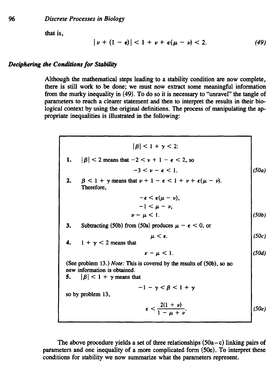
The
above procedure yields
a set of
three relationships
(50a-c)
linking pairs
of
parameters
and one
inequality
of a
more complicated
form
(50e).
To
interpret these
conditions
for
stability
we now
summarize what
the
parameters represent.
(See problem 13.) Note: This
is
covered
by the
results
of
(50b),
so no
new
information
is
obtained.
5.
| ß < 1 + y
means that
3.
Subtracting (5Qb)
from
(50a) produces
/t - e < 0, or
so
by
problem
13,
1. |B| < 2 means that -2
2. B < 1+y means that
Therefore,
4. 1+y < 2 means that
Applications
of
Nonlinear
Difference
Equations
to
Population
Biology
97
We see
that
from
equations
(50a-e)
we can
reach
the
following
conclusions:
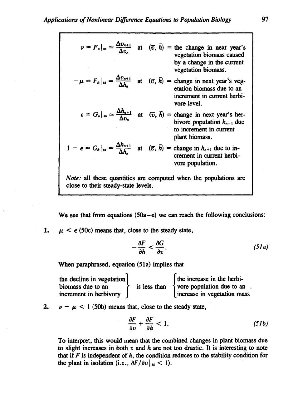
1. fi < e
(50c) means that,
close
to the
steady state,
When paraphrased, equation (5la) implies that
the
decline
in
vegetation
biomass
due to an
increment
in
herbivory
is
less than
the
increase
in the
herbi-
vore population
due to an .
increase
in
vegetation mass
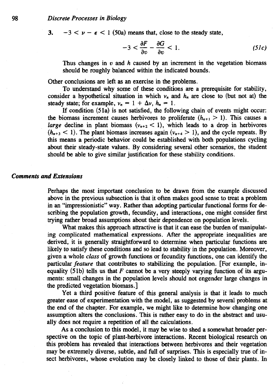
To
interpret, this would mean that
th
bined changes
in
plant biomass
due
to
slight increases
in
both
v and h are not too
drastic.
It is
interesting
to
note
that
if F is
independent
of h, the
condition reduces
to the
stability condition
for
the
plant
in
isolation
(i.e.,
dF/dvls*
< 1).
Note:
all
these quantities
are
computed when
the
populations
are
close
to
their steady-state
levels.
2. v —
fji
< 1
(50b) means that, close
to the
steady state,
the change in next year's
vegetation biomass caused
by a change in the current
vegetation biomass.
Change in next year's veg-
etation biomass due to an
increment in current herbi
vore level.
change in next year's her-
bivore population hn+1 due
to increment in current
plant biomass.
change in hn+1 due to in-
crement in current herbi-
vore population.
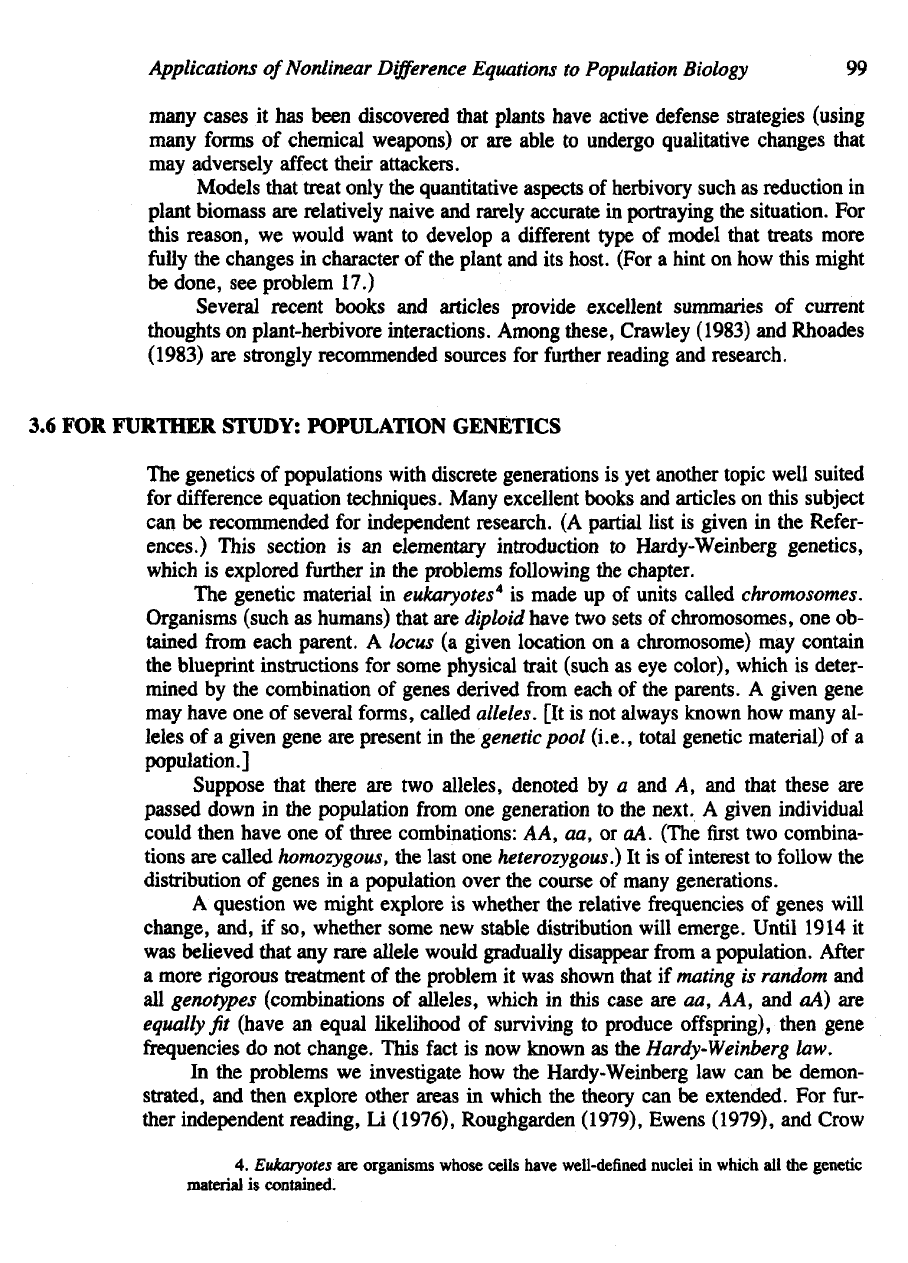
Thus
changes
in v and h
caused
by an
increment
in the
vegetation biomass
should
be
roughly balanced
within
the
indicated bounds.
Other conclusions
are
left
as an
exercise
in the
problems.
To
understand
why
some
of
these conditions
are a
prerequisite
for
stability,
consider
a
hypothetical situation
in
which
v
n
and h
n
are
close
to
(but
not at) the
steady state;
for
example,
v
n
= 1 + Av, h
n
= 1.
If
condition (5la)
is not
satisfied,
the
following chain
of
events might occur:
the
biomass increment causes herbivores
to
proliferate (h
n
+\
> 1).
This causes
a
large
decline
in
plant biomass (v
n+2
< 1),
which leads
to a
drop
in
herbivores
(hn+3
< 1). The
plant biomass increases again
(v
n+4
> 1), and the
cycle repeats.
By
this
means
a
periodic
behavior could
be
established
with
both populations cycling
about
their steady-state values.
By
considering several other scenarios,
the
student
should
be
able
to
give similar justification
for
these stability conditions.
Comments
and
Extensions
Perhaps
the
most important conclusion
to be
drawn
from the
example discussed
above
in the
previous subsection
is
that
it
often
makes good sense
to
treat
a
problem
in
an
"impressionistic" way. Rather
than
adopting particular
functional
forms
for de-
scribing
the
population growth, fecundity,
and
interactions,
one
might consider
first
trying
rather broad assumptions about their dependence
on
population levels.
What makes this approach attractive
is
that
it can
ease
the
burden
of
manipulat-
ing
complicated mathematical expressions.
After
the
appropriate inequalities
are
derived,
it is
generally straightforward
to
determine when particular functions
are
likely
to
satisfy
these conditions
and so
lead
to
stability
in the
population. Moreover,
given
a
whole class
of
growth functions
or
fecundity functions,
one can
identify
the
particular
feature that contributes
to
stabilizing
the
population. [For example,
in-
equality
(5 Ib)
tells
us
that
F
cannot
be a
very steeply varying
function
of its
argu-
ments:
small changes
in the
population levels should
not
engender large changes
in
the
predicted vegetation
biomass.]
Yet
a
third positive
feature
of
this general analysis
is
that
it
leads
to
much
greater
ease
of
experimentation with
the
model,
as
suggested
by
several problems
at
the
end of the
chapter.
For
example,
we
might like
to
determine
how
changing
one
assumption
alters
the
conclusions.
This
is
rather easy
to do in the
abstract
and
usu-
ally
does
not
require
a
repetition
of all the
calculations.
As
a
conclusion
to mis
model,
it may be
wise
to
shed
a
somewhat broader per-
spective
on the
topic
of
plant-herbivore interactions. Recent biological research
on
this problem
has
revealed that interactions between herbivores
and
their
vegetation
may
be
extremely diverse, subtle,
and
full
of
surprises. This
is
especially true
of in-
sect herbivores, whose evolution
may be
closely
linked
to
those
of
their plants.
In
98
Discrete Processes
in
Biology
3.
—
3 < v — e < 1
(50a) means that, close
to the
steady state,
Applications
of
Nonlinear
Difference
Equations
to
Population
Biology
99
many
cases
it has
been
discovered
that plants have active defense strategies (using
many
forms
of
chemical weapons)
or are
able
to
undergo qualitative changes that
may
adversely
affect
their attackers.
Models that treat only
the
quantitative aspects
of
herbivory such
as
reduction
in
plant
biomass
are
relatively naive
and
rarely accurate
in
portraying
the
situation.
For
this reason,
we
would want
to
develop
a
different
type
of
model that treats more
fully
the
changes
in
character
of the
plant
and its
host. (For
a
hint
on how
this might
be
done,
see
problem 17.)
Several recent books
and
articles provide
excellent
summaries
of
current
thoughts
on
plant-herbivore interactions. Among these, Crawley (1983)
and
Rhoades
(1983)
are
strongly recommended sources
for
further
reading
and
research.
3.6
FOR
FURTHER STUDY: POPULATION GENETICS
The
genetics
of
populations with discrete generations
is yet
another topic well suited
for
difference equation techniques. Many excellent books
and
articles
on
this subject
can be
recommended
for
independent research.
(A
partial list
is
given
in the
Refer-
ences.)
This section
is an
elementary introduction
to
Hardy-Weinberg
genetics,
which
is
explored
further
in the
problems following
the
chapter.
The
genetic
material
in
eukaryotes
4
is
made
up of
units called chromosomes.
Organisms (such
as
humans) that
are
diploid
have
two
sets
of
chromosomes,
one ob-
tained
from
each parent.
A
locus
(a
given location
on a
chromosome)
may
contain
the
blueprint instructions
for
some physical trait (such
as eye
color), which
is
deter-
mined
by the
combination
of
genes derived
from
each
of the
parents.
A
given gene
may
have
one of
several forms,
called
alleles.
[It is not
always
known
how
many
al-
leles
of a
given gene
are
present
in the
genetic pool
(i.e.,
total genetic material)
of a
population.]
Suppose
that there
are two
alleles,
denoted
by a and A, and
that these
are
passed
down
in the
population
from
one
generation
to the
next.
A
given individual
could
then have
one of
three combinations:
AA, aa, or aA.
(The
first two
combina-
tions
are
called homozygous,
the
last
one
heterozygous.)
It is of
interest
to
follow
the
distribution
of
genes
in a
population over
the
course
of
many
generations.
A
question
we
might explore
is
whether
the
relative
frequencies of
genes will
change, and,
if so,
whether some
new
stable distribution will emerge. Until 1914
it
was
believed
that
any
rare
allele
would gradually disappear
from
a
population.
After
a
more
rigorous
treatment
of the
problem
it was
shown that
if
mating
is
random
and
all
genotypes
(combinations
of
alleles,
which
in
this case
are aa, AA, and aA) are
equally
jit
(have
an
equal
likelihood
of
surviving
to
produce offspring), then gene
frequencies do not
change.
This
fact
is now
known
as the
Hardy-Weinberg
law.
In
the
problems
we
investigate
how the
Hardy-Weinberg
law can be
demon-
strated,
and
then explore other areas
in
which
the
theory
can be
extended.
For
fur-
ther
independent reading,
Li
(1976), Roughgarden (1979), Ewens (1979),
and
Crow
4.
Eukaryotes
are
organisms whose cells have
well-defined
nuclei
in
which
all the
genetic
material
is
contained.
100
Discrete
Processes
in
Biology
and
Kimura (1970)
are
recommended.
A
mathematical treatment
of the
case
of un-
equal genotype
fitness
is
given
by
Maynard Smith (1968)
and in a
more expanded
form
by
Segel (1984).
To
outline
the
problem, several definitions
and
assumptions
are
needed.
By
convention
we
shall
define
the
frequencies
of the
alleles
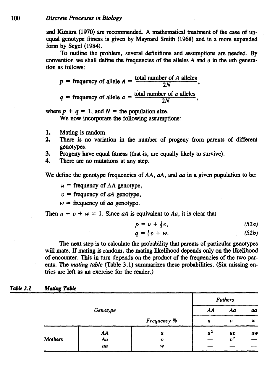
A and a in the nth
genera-
tion
as
follows:
where
p + q = 1, and N = the
population size.
We
now
incorporate
the
following assumptions:
1.
Mating
is
random.
2.
There
is no
variation
in the
number
of
progeny
from
parents
of
different
genotypes.
3.
Progeny have equal fitness (that
is, are
equally likely
to
survive).
4.
There
are no
mutations
at any
step.
We
define
the
genotype frequencies
of AA, aA, and aa in a
given population
to be:
u =
frequency
of
A A
genotype,
v =
frequency
of aA
genotype,
w
-
frequency
of
aa
genotype.
Then
u + v + w = 1.
Since
aA is
equivalent
to Aa, it is
clear that
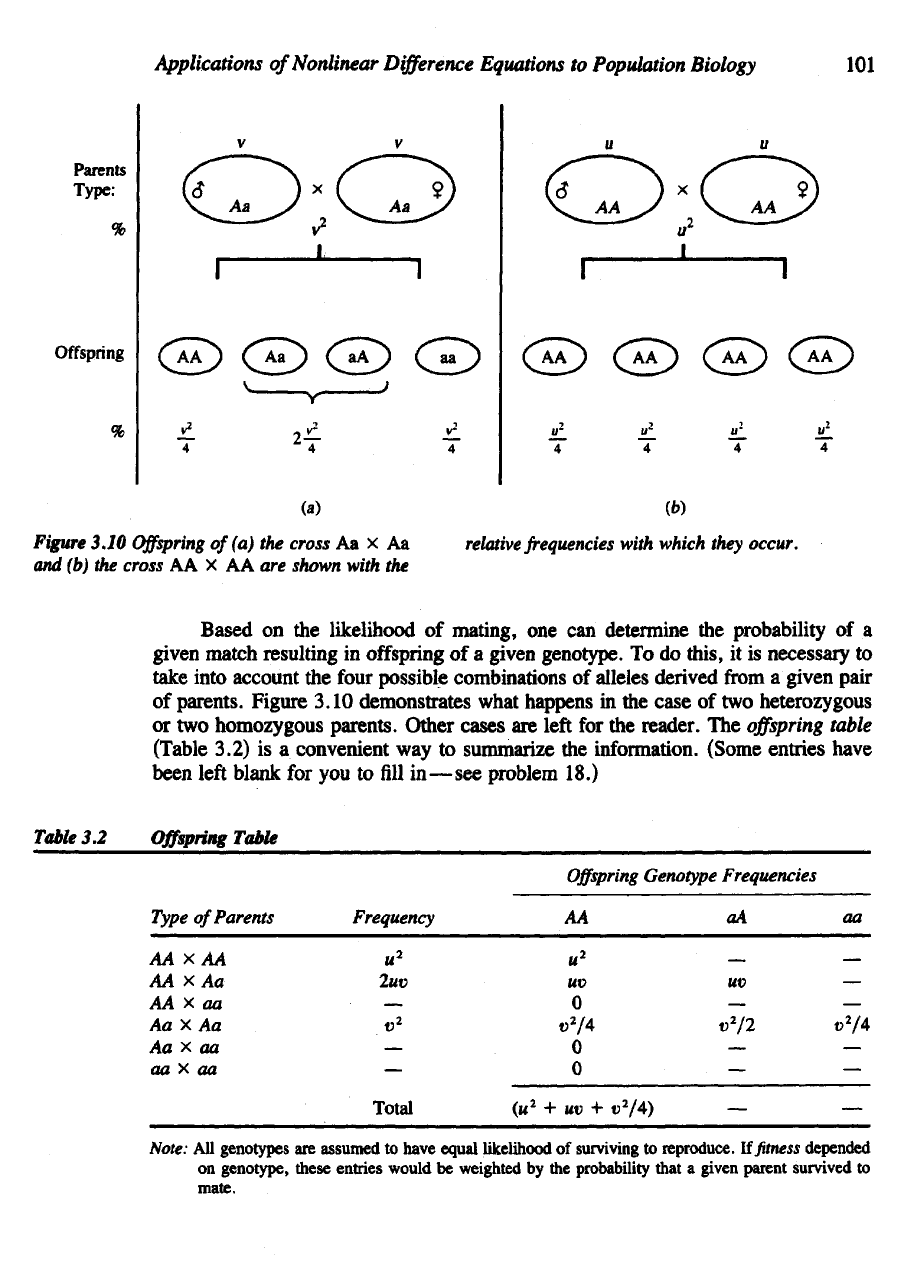
Table
3.1
Mating Table
Genotype
Frequency
%
Mothers
AA
Aa
aa
u
v
w
Fathers
AA Aa
u
v
u
2
uv
- V
2
—
—
aa
w
uw
—
The
next
step
is to
calculate
the
probability that parents
of
particular genotypes
will
mate.
If
mating
is
random,
the
mating likelihood depends only
on the
likelihood
of
encounter. This
in
turn
depends
on the
product
of the
frequencies
of the two
par-
ents.
The
mating
table (Table 3.1) summarizes these probabilities. (Six missing
en-
tries
are
left
as an
exercise
for the
reader.)
Applications
of
Nonlinear
Difference
Equations
to
Population
Biology
101
relative
frequencies
with which they
occur.
Based
on the
likelihood
of
mating,
one can
determine
the
probability
of a
given match resulting
in
offspring
of a
given genotype.
To do
this,
it is
necessary
to
take into account
the
four
possible
combinations
of
alleles
derived
from
a
given pair
of
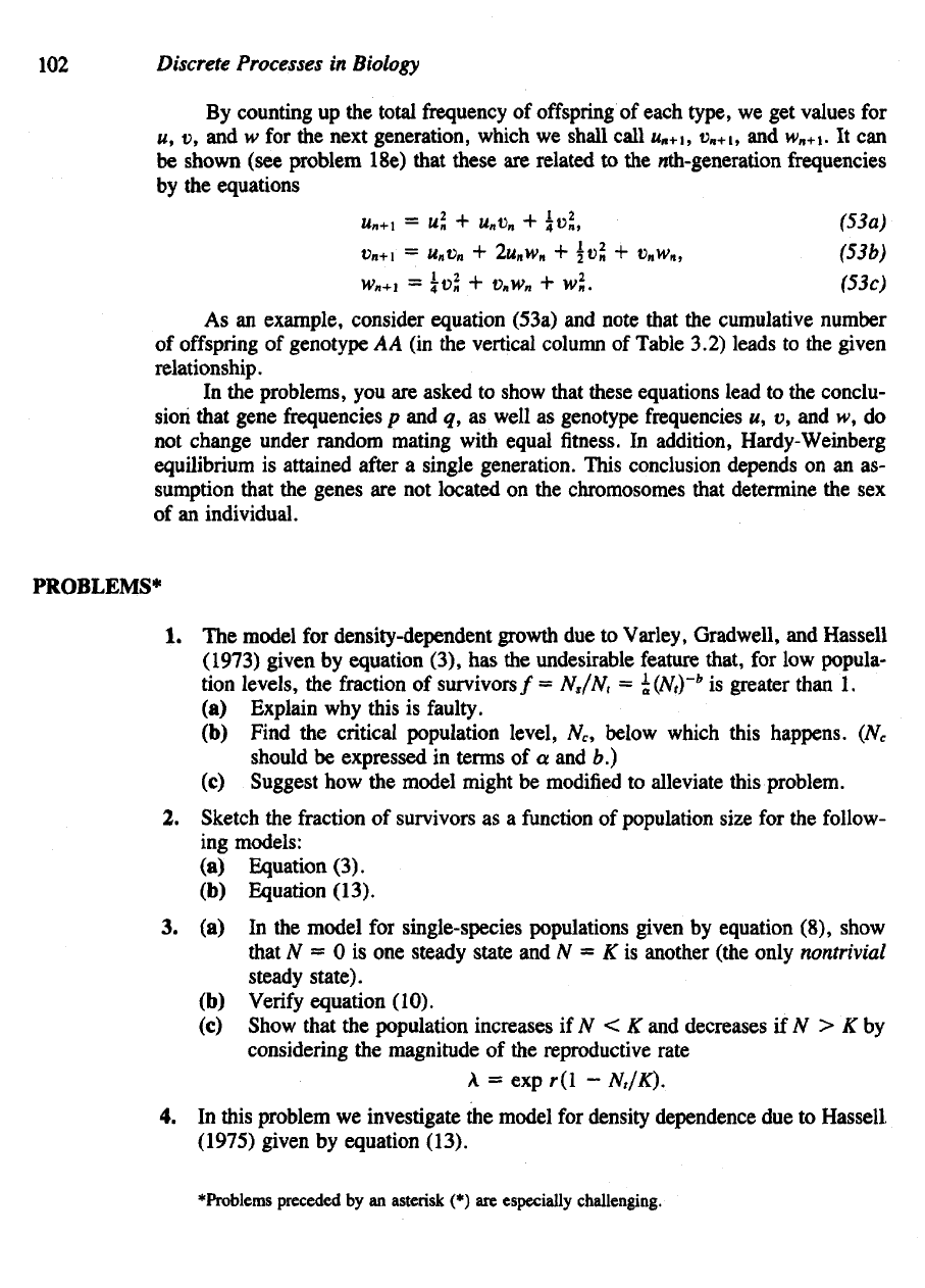
parents. Figure 3.10 demonstrates what happens
in the
case
of two
heterozygous
or two
homozygous parents. Other
cases
are
left
for the
reader.
The
offspring
table
(Table 3.2)
is a
convenient
way to
summarize
the
information. (Some entries have
been
left
blank
for you to fill
in—see
problem 18.)
Table
3.2
Offspring
Table
Offspring
Genotype
Frequencies
Type
of
Parents
AA
x AA
AA X
Aa
AA x aa
Aa
x Aa
Aa
x
aa
aa
x aa
Frequency
«
2
2uv
—
V
—
Total
AA
«
2
uv
0
t?
2
/4
0
0
(M
2
+
Mt3
+
U
2
/4)
oA
__
uv
—
v
2
/2
—
aa
—
—
t)
2
/4
—
Note:
All
genotypes
are
assumed
to
have
equal
likelihood
of
surviving
to
reproduce.
U fitness
depended
on
genotype, these entries
would
be
weighted
by the
probability
that
a
given
parent
survived
to
mate.
Figure
3.10
Offspring
of
(a) the
cross
Aa x Aa
and
(b) the
cross
AA x AA are
shown with
the
102
Discrete Processes
in
Biology
By
counting
up the
total frequency
of
offspring
of
each type,
we get
values
for
M,
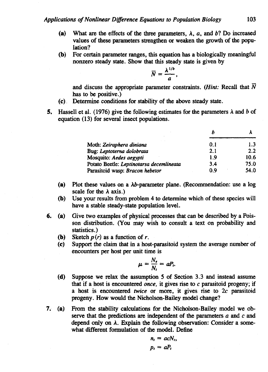
v, and w for the
next generation, which
we
shall call u
n
+\,
tVt-i,
and
w
n
+\.
It can
be
shown (see problem 18e) that these
are
related
to the
/ith-generation frequencies
by
the
equations
PROBLEMS*
1. The
model
for
density-dependent growth
due to
Varley, Gradwell,
and
Hassell
(1973)
given
by
equation (3),
has the
undesirable feature that,
for low
popula-
tion
levels,
the
fraction
of
survivors/
=
N,/N,
=
s(M)~*
is
greater than
1.
(a)
Explain
why
this
is
faulty.
(b)
Find
the
critical population level,
N
c
,
below which this happens.
(N
c
should
be
expressed
in
terms
of a and b.)
(c)
Suggest
how the
model might
be
modified
to
alleviate this problem.
2.
Sketch
the
fraction
of
survivors
as a
function
of
population size
for the
follow-
ing
models:
(a)
Equation (3).
(b)
Equation (13).
3. (a) In the
model
for
single-species
populations given
by
equation (8), show
that
N = 0 is one
steady
state
and N = K is
another (the only nontrivial
steady
state).
(b)
Verify
equation (10).
(c)
Show that
the
population increases
ifN<K
and
decreases
if N > K by
considering
the
ma tude
of the
reproductive rate
4. In
this problem
we
investigate
the
model
for
density dependence
due to
Hassell
(1975)
given
by
equation (13).
"•Problems
preceded
by an
asterisk
(*) are
especially
challenging.
As an
example, consider equation (53a)
and
note
that
the
cumulative number
of
offspring
of
genotype
A A (in the
vertical column
of
Table 3.2) leads
to the
given
relationship.
In
the
problems,
you are
asked
to
show that these equations lead
to the
conclu-
sion
that gene frequencies
p and q, as
well
as
genotype frequencies
u, v, and
H>,
do
not
change under random mating with equal
fitness. In
addition, Hardy-Weinberg
equilibrium
is
attained
after
a
single generation. This conclusion depends
on an as-
sumption that
the
genes
are not
located
on the
chromosomes that determine
the sex
of
an
individual.
Applications
of
Nonlinear
Difference
Equations
to
Population
Biology
103
(a)
What
are the
effects
of the
three parameters,
A, a, and bl Do
increased
values
of
these parameters strengthen
or
weaken
the
growth
of the
popu-
lation?
(b) For
certain parameter ranges, this equation
has a
biologically
meaningful
nonzero steady state. Show that this steady state
is
given
by
b A
Moth:
Zeirapkera diniana
0.1 1.3
Bug: Leptoterna dolobrata
2.1 2.2
Mosquito:
Aedes
aegypti
1.9
10.6
Potato
Beetle:
Leptinotarsa decemlineata
3.4
75.0
Parasitoid
wasp:
Bracon hebetor
0.9
54.0
(a)
Plot these values
on a
A£-parameter pl Recommendation:
use a log
scale
for the A
axis.)
(b) Use
your results
from
problem
4 to
determine which
of
these species will
have
a
stable steady-state population level.
6. (a)
Give
two
examples
of
physical
processes
that
can be
described
by a
Pois-
son
distribution. (You
may
wish
to
consult
a
text
on
probability
and
statistics.)
(b)
Sketch
p
(r)
as a
function
of r.
(c)
Support
the
claim that
in a
host-parasitoid system
the
average number
of
encounters
per
host
per
unit time
is
and
discuss
the
appropriate parameter constraints.
(Hint:
Recall that
N
has to be
positive.)
(c)
Determine conditions
for
stability
of the
above steady state.
5.
Hassell
et al.
(1976)
give
the
following
estimates
for the
parameters
A and b of
equation (13)
for
several insect populations.
(d)
Suppose
we
relax
the
assumption
5 of
Section
3.3 and
instead assume
that
if a
host
is
encountered once,
it
gives
rise to c
parasitoid progeny;
if
a
host
is
encountered
twice
or
more,
it
gives
rise to 2c
parasitoid
progeny.
How
would
the
Nicholson-Bailey model change?
7. (a)
From
the
stability calculations
for the
Nicholson-Bailey model
we ob-
serve that
the
predictions
are
independent
of the
parameters
a and c and
depend only
on A.
Explain
the
following observation: Consider
a
some-
what
different
formulation
of the
model.
Define
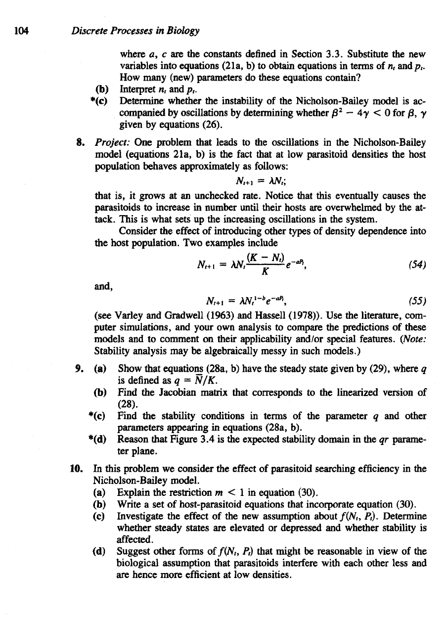
(see Varley
and
Gradwell
(1963)
and
Hassell (1978)).
Use the
literature, com-
puter simulations,
and
your
own
analysis
to
compare
the
predictions
of
these
models
and to
comment
on
their applicability and/or special features.
(Note:
Stability analysis
may be
algebraically messy
in
such models.)
9. (a)
Show that equations (28a,
b)
have
the
steady state given
by
(29), where
q
is
defined
as q —
N/K.
(b)
Find
the
Jacobian matrix that corresponds
to the
linearized version
of
(28).
*(c) Find
the
stability conditions
in
terms
of the
parameter
q and
other
parameters appearing
in
equations (28a,
b).
*(d) Reason that Figure
3.4 is the
expected stability domain
in the qr
parame-
ter
plane.
10. In
this problem
we
consider
the
effect
of
parasitoid searching
efficiency
in the
Nicholson-Bailey model.
(a)
Explain
the
restriction
m < 1 in
equation (30).
(b)
Write
a set of
host-parasitoid equations that incorporate equation (30).
(c)
Investigate
the
effect
of the new
assumption
about/(M,
P
t
). Determine
whether steady states
are
elevated
or
depressed
and
whether stability
is
affected.
(d)
Suggest other
forms
off(N
t
,
P
t
)
that might
be
reasonable
in
view
of the
biological
assumption that parasitoids interfere with each other less
and
are
hence more
efficient
at low
densities.
and,
104
Discrete Processes
in
Biology
where
a, c are the
constants
defined
in
Section 3.3. Substitute
the new
variables into equations (2la,
b) to
obtain equations
in
terms
of n,
and/?,.
How
many (new) parameters
do
these equations contain?
(b)
Interpret
n
t
and pt.
*(c) Determine whether
the
instability
of the
Nicholson-Bailey model
is ac-
companied
by
oscillations
by
determining whether
f3
2
— 4y < 0 for /8, y
given
by
equations (26).
8.
Project:
One
problem that leads
to the
oscillations
in the
Nicholson-Bailey
model (equations 2la,
b) is the
fact
that
at low
parasitoid densities
the
host
population behaves approximately
as
follows:
that
is, it
grows
at an
unchecked rate. Notice
that
this eventually causes
the
parasitoids
to
increase
in
number until their hosts
are
overwhelmed
by the at-
tack. This
is
what sets
up the
increasing oscillations
in the
system.
Consider
the
effect
of
introducing other types
of
de ity dependence into
the
host population.
Two
examples include
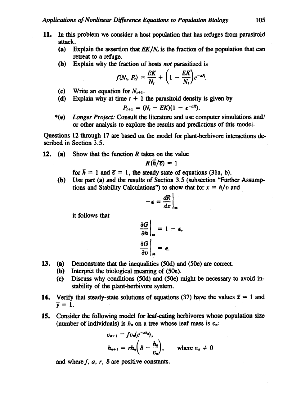
Applications
of
Nonlinear
Difference
Equati
105
11. In
this problem
we
consider
a
host po parasitoid
attack.
(a)
Explain
the
assertion that
EK/N,
is the
fraction
of the
population that
can
retreat
to a
refuge.
(b)
Explain
why the
fraction
of
hosts
not
parasitized
is
(c)
Write
an
equation
for
N
t
+i.
(d)
Explain
why at
time
t + 1 the
parasitoid density
is
given
by
13. (a)
Demonstrate that
the
inequalities
(50d)
and
(SOe)
are
correct.
(b)
Interpret
the
biological meaning
of
(SOe).
(c)
Discuss
why
conditions
(50d)
and
(SOe)
might
be
necessary
to
avoid
in-
stability
of the
plant-herbivore system.
14.
Verify
that steady-state solutions
of
equations (37) have
the
values
x
= 1 and
y
=
1-
15.
Consider
the
following model
for
leaf-eating herbivores whose population
size
(number
of
individuals)
is
h
n
on a
tree whose leaf mass
is
v
n
:
for
h — 1 and v = 1, the
steady state
of
equations
(3la,
b).
(b) Use
part
(a) and the
results
of
Section
3.S
(subsection "Further Assump
tions
and
Stability Calculations")
to
show that
for x = h/v and
*(e) Longer
Project:
Consult
the
literature
and use
computer simulations and/
or
other analysis
to
explore
the
results
and
predictions
of
this model.
Questions
12
through
17 are
based
on the
model
for
plant-herbivore interactions
de-
scribed
in
Section
3.5.
. (a)
Show that
the
function
R
takes
on the
value
and
wher
, r, 6 are
positive
constants.
it
follows that
